String Similarity Metrics – Edit Distance | Baeldung on Computer Science

1. Introduction

In this tutorial, we’ll learn about the ways to quantify the similarity of strings. For the most part, we’ll discuss different string distance types available to use in our applications. We’ll overview different metrics and discuss their properties and computational complexity for each method. Finally, we’ll come up with the recommendations on technique selection for a specific data set.

2. Problem Context and Metric Categories

Multiple applications – ranging from record linkage and spelling corrections to speech recognition and genetic sequencing – rely on some quantitative metrics to determine the measure of string similarity. String similarity calculation can help us with any of these problems but generally computationally expensive and don’t automatically produce ideal outcomes due to the diverse and fuzzy nature of all the possible data faults.

Given this, we may want to select the optimal metrics to use from the entire set of available techniques. Below is the chart of the most common string similarity distance metrics grouped into 4 categories:

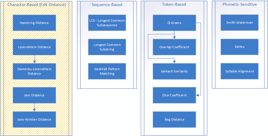
In this article, we’re going to discuss the first category, focused on direct character comparison in strings. All of the metrics in this family are derived from the number of edit operations executed on strings, hence commonly referred to as edit distances.

3. Hamming Distance

Hamming distance is the number of positions at which the corresponding symbols in compared strings are different. This is equivalent to the minimum number of substitutions required to transform one string into another.

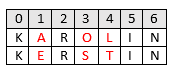
Let’s take two strings, KAROLIN and KERSTIN. We may observe that the characters at positions 1, 3, and 4 (zero-based) are different, with all the rest being equivalent.

This means Hamming distance is 3 in this case:

The easiest of all the string distance metrics, Hamming distance, applies to the strings of the same length only. Computation is trivial with linear time complexity.

4. Levenshtein Distance

Levenshtein distance, like Hamming distance, is the smallest number of edit operations required to transform one string into the other. Unlike Hamming distance, the set of edit operations also includes insertions and deletions, thus allowing us to compare strings of different lengths.

Given two strings, the Levenshtein distance between them is the minimum number of single-character edits (insertions, deletions, or substitutions) required to change one string into the other.

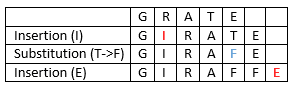
For example, the Levenshtein distance between GRATE and GIRAFFE is 3:

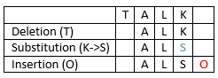
If two strings have the same size, the Hamming distance is an upper bound on the Levenshtein distance. For example, the Hamming distance of TALK and ALSO is 4 since the characters at each location are different. However, their Levenshtein distance is only 3:

Levenshtein distance conforms to metric requirements, most importantly being symmetric and satisfying triangle inequality:

$dist(a, b) = dist (b, a)$

$dist(a, b) \leq dist(a, c) + dist(b, c)$

Levenshtein distance computation can be costly, worst-case complete calculation has $\mathcal{O}( |a| \times |b| )$ time complexity and $\mathcal{O}( min(|a|,|b|) )$ space complexity. A number of optimization techniques exist to improve amortized complexity but the general approach is to avoid complete Levenshtein distance calculation above some pre-selected threshold.

If we want to use normalized metric, we may convert Levenshtein distance to similarity measure using the formula:

$sim_{ld}(a, b) = 1.0 - \dfrac{dist(a, b)}{max(|a|, |b|)}$

5. Damerau-Levenshtein Distance

It has been observed that most of the human misspelling errors fall into the errors of these 4 types – insertion, deletion, substitution, and transposition. Motivated by this empirical observation, Damerau-Levenshtein distance extends the set of the edit operations allowed in Levenshtein distance with transposition of two adjacent characters.

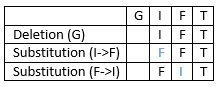
For example, the Levenshtein distance between GIFT and FIT is 3:

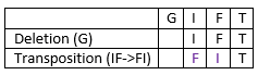
In this example, we need two steps to transform IF into FI. However, if we allow transposition between two adjacent characters, we can use only one step to make the transformation. Therefore, the Damerau-Levenshtein distance between GIFT and FIT is 2:

Incorporating transposition into the original Levenshtein distance computation algorithms can be relatively challenging. Straightforward modification of the dynamic programming approach used for Levenshtein distance computation with the entry responsible for transposition unexpectedly calculates not Damerau-Levenshtein distance but “optimal string alignment distance” which is not only different from the expected result but also doesn’t hold triangle inequality property.

Efficient algorithms to calculate Damerau-Levenshtein distance provide the same time complexity – $\mathcal{O}( |a| \times |b| )$ .

6. Jaro Distance

The Jaro similarity between strings $a$ and $b$ is defined using the formula:

$sim_{j}= \begin{cases} 0 \hfill \mbox{ if } m=0, \\ \dfrac{1}{3} \left( \dfrac{m}{|{a}|} + \dfrac{m}{|{b}|} + \dfrac{m - t}{m} \right) \hfill \mbox{ otherwise} \\ \end{cases}$

Where:

$m$ is the number of matching characters. We consider two characters from $a$ and $b$ as matching if they are the same and not farther than ${\left\lfloor {\frac {\max(|{a}|,|{b}|)}{2}}\right\rfloor -1$ characters apart.

$t$ is half the number of matching (but different sequence order) characters.

The Jaro similarity value ranges from 0 to 1 inclusive. If two strings are exactly the same, then $|{a}| = |{b}| = m$ and $t=0$ . Therefore, their Jaro similarity is 1 based on the second condition. On the other side, if two strings are totally different, then $m=0$ . Their Jaro similarity will be 0 based on the first condition.

The Jaro distance is the inversion of Jaro similarity: $1-sim_{j}$ . Therefore, a larger Jaro distance value means more difference between two strings.

For example, comparing CARTEL vs. TRACE, we may see that only ‘A’, ‘R’, and ‘E’ are the matching characters:

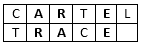
The matching distance threshold is ${\left\lfloor {\frac {\max(6, 5)}{2}}\right\rfloor -1 = 2$ . Although character ‘C’ appears in both strings, they are 3 characters apart. Therefore, we don’t consider ‘C’ as the matching character. Similarly, the character ‘T’ is also not a matching character. Overall, the total number of matching characters is $m=3$ .

The matching sequences are ARE and RAE. The number of matching (but different sequence order) characters is 2, which means $t=1$ . Theorefore, the Jaro similarity value of the two strings is $\dfrac{1}{3} \left( \dfrac{3}{6} + \dfrac{3}{5} + \dfrac{3 - 1}{3}\right) = \dfrac{53 }{90} \approx 0.5889$ . Then, the Jaro distance is $1 - \dfrac{53 }{90} \approx 0.4111$ .

The time complexity is quadratic while the space complexity of the algorithm to compute Jaro distance is $\mathcal{O}(|a| + |b|)$ .

7. Jaro-Winkler Distance

Winkler improved the Jaro algorithm by applying ideas based on empirical observations, which found that fewer errors typically occur at the beginning of misspelled person names.

The Winkler algorithm, therefore, increases the Jaro similarity measure for equivalent initial characters:

$sim_{jw}(a, b) = sim_{j}(a, b) + l * p * (1 - sim_{j}(a, b))$

Where:

$l$ is the length of the common prefix at the start of both strings, up to a maximum of 4.

$p$ is the scaling factor. The scaling factor shouldn’t exceed 0.25. Otherwise, the similarity may become larger than 1 as the maximum length of the considered prefix is 4. Original Winkler’s work used value 0.1.

Similar to Jaro distance, we can define Jaro-Winkler distance as $d_{jw}=1-sim_{jw}$ .

For example, when we compare two strings TREAT and TRACE, the matching sequence is TRA:

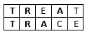
Therefore, the Jaro similarity between these two strings is $\dfrac{1}{3} \left( \dfrac{3}{5} + \dfrac{3}{5} + \dfrac{3 - 0}{3}\right) = \dfrac{11 }{15} \approx 0.7333$ . The common prefix of the two strings is TR, which has length of 2. If we use 0.1 as the scaling factor, the Jaro-Winkler similarity will be $\dfrac{11 }{15} + 2 * 0.1 * (1 - \dfrac{11 }{15}) = \dfrac{59 }{75} \approx 0.7867$ . Then, the Jaro-Winkler distance is $1 - \dfrac{59}{75} \approx 0.2133$ .

Jaro–Winkler distance doesn’t obey the triangle inequality and hence isn’t a metric suitable to build metric space.

Winkler also considered the topic of comparing the strings having two or more words, possibly differently ordered. To this end, he introduced the variants Sorted Winkler and Permuted Winkler. The former algorithm alphabetically sorts strings before calculating their similarity, while the latter calculates the similarity over all possible permutations and returns the maximum value.

8. Evaluation and Recommendations

Given all the variety of available algorithms, it becomes important to evaluate matching quality on relevant data sets. The final result of any match should be classified as match/non-match based on the selected similarity measure threshold – string pairs with a similarity value above the threshold are classified matches, and pairs with similarity value below as non-matches.

To provide tangible estimation, the common practice is to use labeled training data.

For every matching pair, we define the number of the true positives $TP$ – known matched string pairs classified as matches, the true negatives $TN$ – known un-matched pairs classified as non-matches, the false positives $FP$ – unmatched pairs classified as matches, and the false negatives $FN$ – known matched pairs classified as non-matches.

Using these values, we estimate Precision and Recall:

$P = \dfrac{TP}{TP + FP}$

$R = \dfrac{TP}{TP + FN}$

Precision reflects the share of real correspondences among all found matches. A solution having a high value of precision means that it doesn’t return many false positives.

Recall specifies the share of real correspondences. A high value of recall of a given solution means that it doesn’t return many false negatives.

Finally, to estimate overall efficiency, we may use F-measure. F-measure is the harmonic mean of precision and recall:

$R = \dfrac{2 \times P \times R}{P + R}$

Selecting the optimal threshold to achieve the highest F-measure may prove to be challenging. Some algorithms and data sets have low coupling between the similarity measure threshold and resulting F-measure, while others demonstrate that even small threshold changes can result in dramatic drops in matching quality.

Besides matching quality, performance is crucial to process large data sets.

If speed is important, it is imperative to use techniques with time complexity linear in the string length. If it is known that the name data at hand contains a large proportion of nicknames, aliases, and similar variations, a dictionary-based name standardization should be applied before performing the matching.

Generally, we may want to use heavy algorithms providing better quality – like Levenshtein distance – for shorter strings, and token-based – like q-grams or bag distance – for longer strings.

Besides the similarity of strings, syntactical by nature, we may need to address the related problem of finding the semantical similarity in different sentences or entire documents. There’s a variety of semantic metrics based on Path Length, Information Content, Dictionaries, and more. On top of them, several statistical approaches have been built, including Latent Semantic Analysis, Pointwise Mutual Information, and many more.

There’re some other, less common metrics outside of the categories outlined above as well, like NCD – Normalized Compression Distance, which you may want to employ in your application.

9. Conclusion

In this tutorial, we’ve discussed multiple algorithms and metrics to evaluate string similarity.

We found that we may use multiple different approaches to address this problem, each of them having its own complexity, in terms of both the implementation and the execution.

Finally, we’ve seen how we can evaluate these metrics to find the best fit for our application.

Full Archive

About Baeldung

Core Concepts

Operating Systems

Artificial Intelligence

Graph Theory

Latex