Binary Search Trees vs. AVL Trees: the Complexity of Construction

1. Introduction

In this tutorial, we’ll explain the difference in time complexity between binary-search and AVL trees. More specifically, we’ll focus on the expected and worst-case scenarios for constructing the trees out of arrays.

When it comes to space complexity, both trees require $O(n)$ space to be constructed regardless of the case analyzed.

2. Binary Search Trees and AVL Trees

In a binary search tree (BST), each node’s value is $<$ than its left descendants’ values and $\leq$ than the values in its right sub-tree.

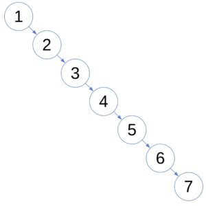
The goal of BSTs is to allow efficient searches. Although that’s mostly the case, the caveat is that a BST’s shape depends on the order in which we insert its nodes. In the worst case, a plain BST degenerates to a linked list and has an $O(n)$ search complexity:

Balanced trees were designed to overcome that issue. While building a balanced tree, we maintain the shape suitable for fast searches. In particular, when it comes to AVL trees, the heights of each node’s left and right sub-trees differ at most by 1:

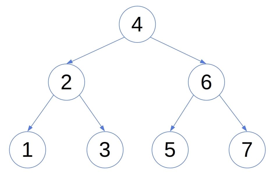
That property implies that an AVL tree’s height is $\boldsymbol{O(\log n)}$ . To ensure it, we need to re-balance the tree if an insertion unbalances it, which incurs computational overhead.

Here, we’ll analyze the complexity of building an AVL tree and a BST out of an array $A$ of comparable objects: $A = [a_1, a_2, \ldots, a_n]$

3. The Worst-Case Complexity Analysis

Let’s first analyze the worst-case scenario. For both BST and AVL trees, the construction algorithms follow the same pattern:

The algorithm starts with an empty tree and inserts the elements of $A$ successively until processing the whole array. To place $a_i$ , the algorithm first looks for it in the tree containing $a_1, a_2, \ldots, a_{i-1}$ . The search procedure identifies the node $x$ whose child $a_i$ should become. Then, the algorithm inserts $a_i$ as the left or right child of $x$ depending on whether $a_i < x.value$ or $a_i \geq x.value$ .

3.1. Constructing a BST

In the worst-case scenario, when the insertion order $a_1 \leq a_2 \leq \ldots \leq a_n$ skews the tree, the insertion into a BST is a linear-time operation.

Since the tree is essentially a list, adding $a_i$ to the tree in the worst case requires traversing all the previously attached elements: $a_1 , a_2, \ldots a_{i-1}$ . In total, we follow $\boldsymbol{O(n^2)}$ pointers:

(1) $\begin{equation*} \sum_{i=1}^{n} (i-1) = \sum_{i=0}^{n-1} i = \frac{n(n-1)}{2} \in O(n^2) \end{equation*}$

So, constructing a BST takes a quadratic time in the worst case.

3.2. Constructing an AVL Tree

Insertion into an AVL tree takes log-linear time. The reason is that an AVL tree’s height is logarithmic in the number of nodes, so we traverse no more than $O(\log i)$ edges when inserting $a_i$ in the worst case. In total:

(2) $\begin{equation*} \sum_{i=1}^{n} O(\log i) = \sum_{i=1}^{n} \underbrace{O(\log n)}_{\text{since } i \leq n} = O(n \log n) \end{equation*}$

The worst-case complexity of building an AVL tree is $\boldsymbol{O(n \log n)}$ . So, although insertions can trigger re-balancing, an AVL tree is still faster to build than an ordinary BST.

4. The Expected Complexity

In the following analyses, we assume that all $n!$ insertion orders of $A=[a_1, a_2, \ldots, a_n]$ are equally likely.

4.1. Binary Search Trees

A single insertion’s complexity depends on the average node depth in a BST. We can calculate it as the sum of the nodes’ depths divided by the number of nodes ( $n$ ).

If the root’s left sub-tree has $i$ nodes, the right one contains $n-i$ vertices. Then, the expected sum of the depths in such a BST, $D(n, i)$ , is:

(3) $\begin{equation*} D(n, i) = n-1 + D(i) + D(n-i-1) \qquad (D(1)=0) \end{equation*}$

We add $n-1$ because the root node increases the depths of all the other nodes by 1.

Since all permutations of $A$ are equally probable, $i$ follows the uniform distribution over $\{0, 1, \ldots, n-1\}$ . So, the expected depth of a node in a BST with $n$ nodes is:

(4) $\begin{equation*} D(n) = \frac{1}{n}\sum_{i=0}^{n-1} D(n, i) = n-1 + \frac{2}{n}\sum_{i=0}^{n}D(i) \end{equation*}$

Solving the recurrence, we get $D(n) \in O(n \log n)$ . So, the expected node depth in a BST with $n$ nodes is $O(\log n)$ . Hence, starting from an empty tree and inserting $a_1, a_2, \ldots, a_n$ , we perform $O(n \log n)$ steps:

(5) $\begin{equation*} \sum_{i=2}^{n} O(\log (i-1)) = \sum_{i=2}^{n} \underbrace{O(\log n)}_{\text{since } i -1 \leq n} = O(n \log n) \end{equation*}$

Therefore, in the average case, the construction of a BST takes a log-linear time.

4.2. AVL Trees

Since the AVL trees are balanced and do not depend on the insertion order, the tree depth is always $O(\log n)$ . Moreover, an AVL tree has at most $2^k$ nodes at depth $k$ . So, the average node depth is bounded by:

(6) $\begin{equation*} \frac{1}{n}\sum_{k=0}^{O(\log n)}k 2^k \end{equation*}$

Since:

$\sum_{k=0}^{d} k 2^k = 2^{d+1}(d-1)+2$

the expected node depth in an AVL tree is:

(7) $\begin{equation*} O \left( \frac{1}{n} 2^{\log n + 1}(\log n - 1) + 2 \right) = O \left( \frac{1}{n} n \log n \right) = O(\log n) \end{equation*}$

Since the average node depth is the same as in a BST, Equation (5) holds for AVL trees as well. So, building an AVL tree is also a log-linear operation in the expected case.

5. Conclusion

In this article, we compared the construction complexities of Binary Search Trees (BSTs) and AVL trees. In the worst-case scenario, building an AVL tree takes $O(n \log n)$ time, whereas constructing a BST has an $O(n^2)$ complexity.

However, both trees take a log-linear time in the expected case.

Full Archive

About Baeldung

Core Concepts

Operating Systems

Artificial Intelligence

Graph Theory

Latex