

Learn through the super-clean Baeldung Pro experience:
>> Membership and Baeldung Pro.
No ads, dark-mode and 6 months free of IntelliJ Idea Ultimate to start with.
Learn through the super-clean Baeldung Pro experience:
>> Membership and Baeldung Pro.
No ads, dark-mode and 6 months free of IntelliJ Idea Ultimate to start with.
A tree is a fundamental data structure that possesses a lot of desirable characteristics. We can search a tree quickly as in an ordered array, and we also have a quick insert and delete as in a linked list.
In this article, we’ll review the different types of tree structures as well as some main differences among them.
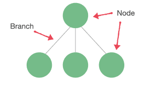
When we think of trees, we immediately think of roots, branches, and leaves. Well, this is exactly what the anatomy of a tree looks like in Computer Science.
A tree consists of a series of nodes (vertices) completely connected by what we call branches (edges). These branches don’t possess any direction:
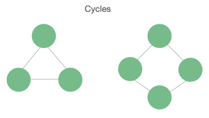
Branches must not create any cycles between the different nodes. If we find cycles in the structure, then we are not dealing with a tree:
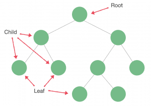
Trees work based on a hierarchical structure, meaning we’ll have parent nodes and child nodes. A tree has only one root node.
Each node can only have one parent but it can have multiple children. A node without a child is called a leaf. A node can have null children as well:
The most common place where we can find an instance of a tree is in the folder structure of our file system.
Other important concepts of a tree are:
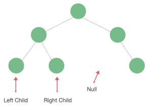
A Binary Tree is a type of tree where each node can have no more than two child nodes.
Every node in a Binary Tree possesses a value, a right child, a left child, and a parent. Left and right child nodes may be null:
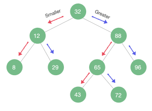
A Binary Search Tree (BST) is a more specific type of Binary Tree where the main characteristic is that it’s sorted.
A Binary Tree is a BST if and only if an inorder traversal of the binary tree results in a sorted sequence.
On any subtree of a BST, the nodes to the left of the parent node are smaller than it, and the nodes to the right of a parent node are greater than it:
Average time complexity:
Let’s check the insertion pseudocode of a Binary Search Tree:
algorithm BSTInsert(n, t):
    // INPUT
    //   n = Node to insert
    //   t = Binary Search Tree
    // OUTPUT
    //   Inserts the given node into the BST

    temp <- null
    current <- t.root

    while current != null:
        temp <- current
        if n.val < current.val:
            current <- current.left
        else:
            current <- current.right

    n.parent <- temp

    if temp = null:
        t.root <- n
    else if n.val < temp.val:
        temp.left <- n
    else:
temp.right <- nIf data is unevenly distributed along the tree, we’ll end up with an unbalanced tree. While inserting elements into our tree, if we do the insertion from a mostly ascending or descending sequence, our tree will have most of its nodes on one side of the root and few in the other.
In fact, we’ll face the worst-case scenario if we insert elements into our tree from an already sorted list:
data = [8, 12, 29, 43, 65]
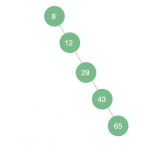
As we can see, if our tree is unbalanced and we deal with the worst-case scenario, it will look like a LinkedList.
Average time complexity:
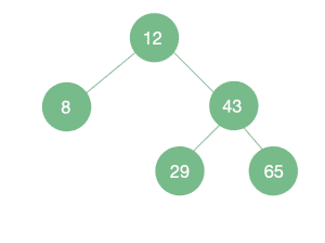
If we insert elements into our BST randomly, the tree will be more or less balanced.
There are different ways to achieve a Balanced BST. One way would be to randomize our original dataset before inserting it:
data = [12, 43, 65, 8, 29]
Average time complexity:
Next, let’s check some of the ways to maintain a balanced tree.
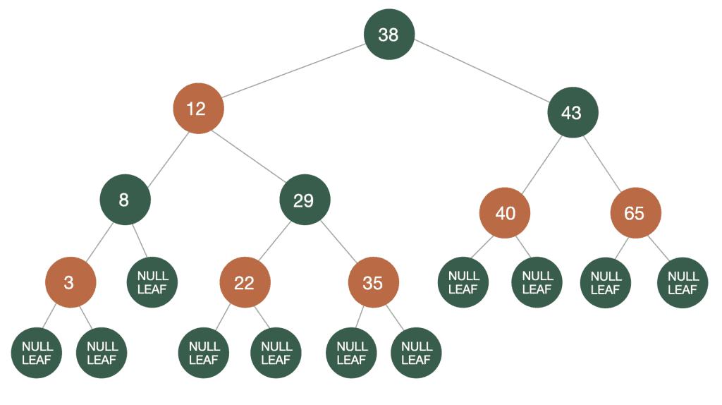
Red-Black Trees are one of several self-balanced tree structures. In a Red-Black Tree, in addition to the usual Binary Tree properties, each node contains the extra property Color. This color can be either red or black, and it is used to add a set of rules, called the red-black rules, that are used for balancing the tree:
We call the number of black nodes on a path from a node to a leaf the black height of the node. Rephrasing rule 4, we can also say that the black height must be the same for all paths from the root to a leaf:
Average time complexity:
The AVL Tree was the first self-balancing tree to be introduced. It received its name after its inventors: Andelson-Velskii and Landis.
In AVL Trees, the nodes hold an extra property, which is the difference in height between the left and right subtrees. This is called the balancing factor.
The balancing factor on an AVL Tree shouldn’t be greater than 1 for any node.
After an insertion or deletion of a node, our tree is potentially unbalanced. If the balancing factor differs by more than 1, a rotation is needed to normalize the heights.
Average time complexity:
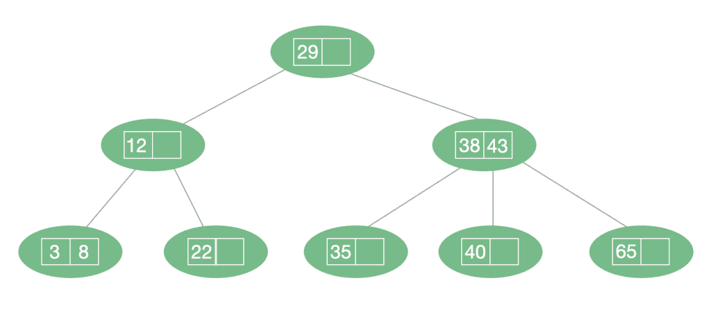
A B-Tree is a type of multiway tree. Multiway trees can have more than two child nodes — in fact, they can contain from a few to thousands of them.
One problem with multiway trees is that each node must be larger than for a binary tree since it contains more data and needs to hold a reference to every one of its children.
B-trees are similar to Red-Black trees, but they are particularly useful for organizing data in external storage.
In a B-Tree, each node will contain n keys and it will have n+1 children. Thus, all of its leaves are at the same depth.
The restrictions of B-Trees make them perfectly balanced. They are also at least half full and contain few levels:
Average time complexity:
In this article, we explored some of the different types of tree structures and the particular characteristics of each.
When ready to jump into further implementation details, be sure to check our article, Implementing a Binary Tree in Java.