

Learn through the super-clean Baeldung Pro experience:
>> Membership and Baeldung Pro.
No ads, dark-mode and 6 months free of IntelliJ Idea Ultimate to start with.
Learn through the super-clean Baeldung Pro experience:
>> Membership and Baeldung Pro.
No ads, dark-mode and 6 months free of IntelliJ Idea Ultimate to start with.
In this tutorial, we’ll discuss two self-balancing binary data structures: AVL and red-black tree. We’ll present the properties and operations with examples.
Finally, we’ll explore some core differences between them.
To understand AVL trees, let’s first discuss the binary tree data structure. It’ll help us understand why we need the AVL tree data structure.
In a binary tree data structure, there can be a maximum of two children nodes allowed. Using a binary tree, we can organize data. However, data is not well optimized for searching or traversing operations.
Therefore, the binary search tree (BST) data structure is introduced to overcome this issue. It’s an updated version of a binary tree. The extra added property is that the data which is smaller than the parent node will be added to the left subtree. Similarly, if the information is greater than the parent node, we add them to the right subtree.
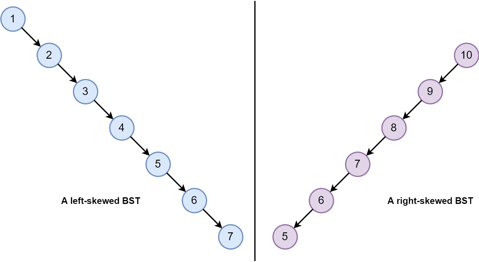
All the tree operations are optimized in a binary search tree, and execution time is faster than a binary tree. But still, it has some issues. A binary search tree can become a left-skewed or right-skewed tree. Let’s look at a left-skewed and right-skewed tree:
The best benefit of the BST data structure is the time complexity of all the tree operations is  , where
  is the number of total nodes. Although when a BST is a left-skewed or right-skewed tree, time complexity becomes
  . The solution to this issue is the AVL tree data structure.
It’s a type of self-balancing binary search tree. There’s a balance factor for each node, and it must be  , or
, or  . The balance factor is calculated by subtracting the height of the right subtree from the height of the left subtree. If the balance factor is greater than
  or
or  , we need to apply rotations to rebalance the tree. Let’s look at an AVL tree:
AVL tree has a balance factor which ensures that the time complexity for tree operations should be  in the average as well as in the worst case.
Now let’s talk about the properties of the AVL tree data structure.
AVL tree is also known as the height-balanced tree. The maximum number of nodes in an AVL tree of height  can be
  . Additionally, the minimum number of nodes in an AVL tree of height
  can be calculated using recurrence relation:
  , where
  , and
, and  .
.
We can balance an AVL tree by applying the left or right rotation. The tree operations on the AVL tree work the same as the BST. However, after performing any tree operations, we need to check the balance factor for each node. Therefore, if the tree is unbalanced, we perform rotations in order to make it balanced.
The elements in the right subtree may increase, and the AVL tree can become unbalanced after applying some tree operations. We rotate the unbalanced node to the left side to overcome this to make the AVL tree balanced again.
The elements in the left subtree may increase, and the AVL tree can become unbalanced after applying some tree operations. To overcome this, we rotate the unbalanced node to the right side to make the AVL tree balanced again.
Another possibility is when we perform some tree operations in the AVL tree, and it becomes unbalanced with no right subtree, but the left subtree contains all the nodes whose value is greater than their parent node. To overcome this, we have to perform two rotations, one right rotation, and one left rotation.
Similarly, an AVL tree can become unbalanced with no left subtree, but the right subtree only contains nodes whose value is less than their parent node. We have to perform two rotations to balance the AVL tree: one left rotation and a right rotation.
Because every AVL tree is a BST, the searching operation in the AVL tree is similar to the BST. We start the searching process by comparing the element we want to find with the root node. Moreover, based on the required element’s key value, we go either left or right subtree from the root node and repeat the process. We terminate the search process when locating the required element or fully exploring the tree.
The time complexity for searching an element in the AVL is , where the total number of nodes in an AVL tree is .
Insertion operation in the AVL tree is similar to the BST insertion. Although, in the AVL tree, there is an additional step. We need to calculate the balance factor for each node after the insertion operation to ensure the tree is always balanced. Let’s discuss the steps of the insertion operation.
If the tree is empty, insert the element at the root. If the tree is not empty, then we first compare the value of the node we want to insert with the parent or root node. Based on the comparison, we either go to the right or left subtree and get the appropriate location for inserting the new node.
After the insertion process, we calculate the balance factor for each node. If any node is unbalanced, we perform some rotations as per the requirement until the tree becomes balanced again. The time complexity for the insertion process in the AVL tree is .
Let’s look at an example. We want to insert a set of nodes in the AVL tree with given key values:  . Initially, the tree is empty. We’ll inset nodes one by one.
First, we insert a node with a key of  . It would be the root node of the AVL tree. Now, let’s insert the node with key
  followed by the node with key
  . After inserting the nodes, we also calculate the balance factor for each node:
Now let’s insert the nodes with key values  and
and  :
:
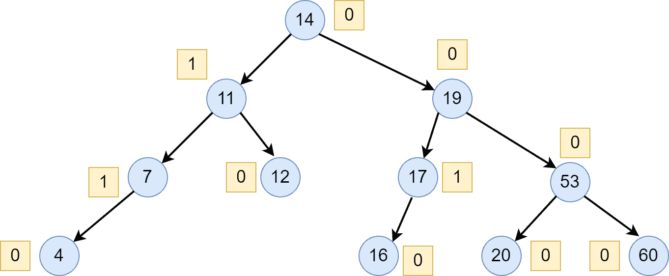
Till now, we have a balanced AVL tree. Hence, we don’t need to perform any rotations. Let’s insert the next node with a key-value  :
:
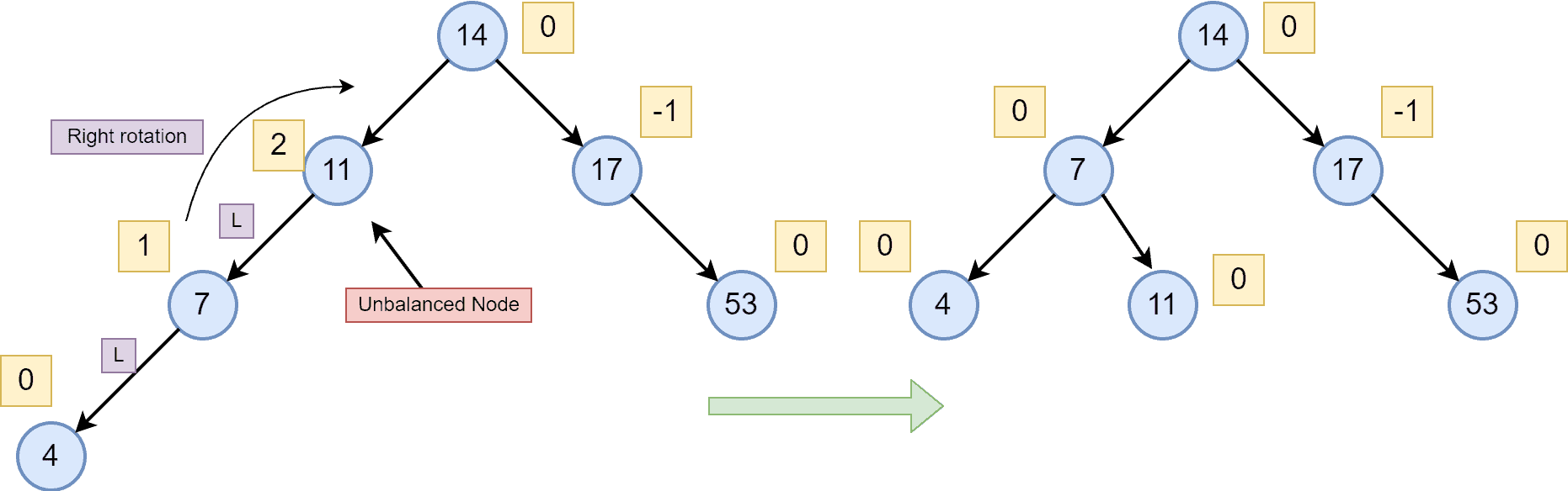
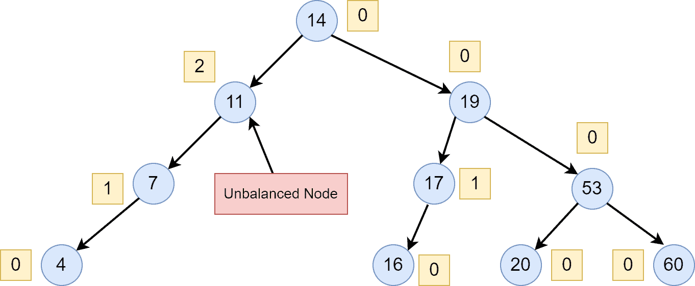
As we can see, after inserting the node with the key-value , the tree becomes unbalanced. Hence, we have performed a left rotation in order to rebalance the tree. Let’s insert the next node with key-value  :
:
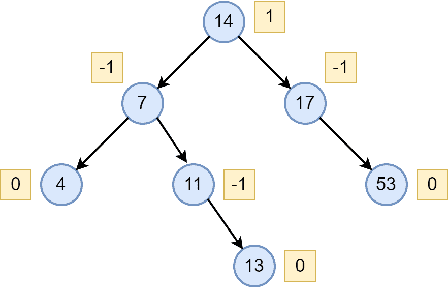
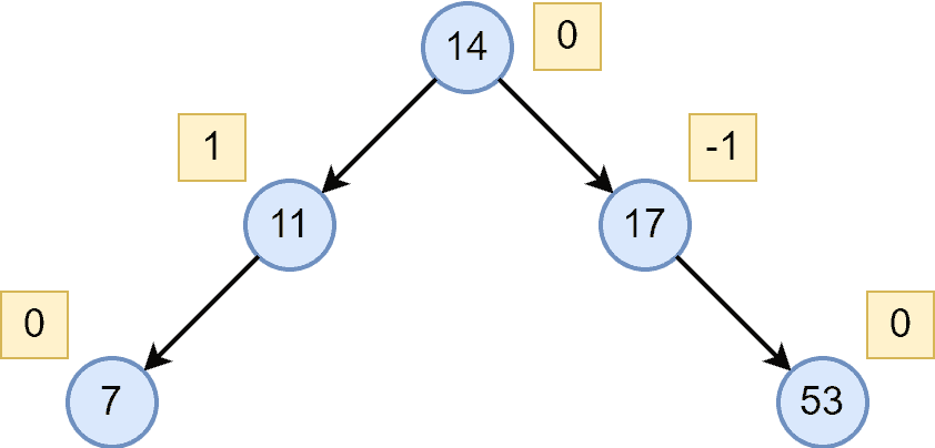
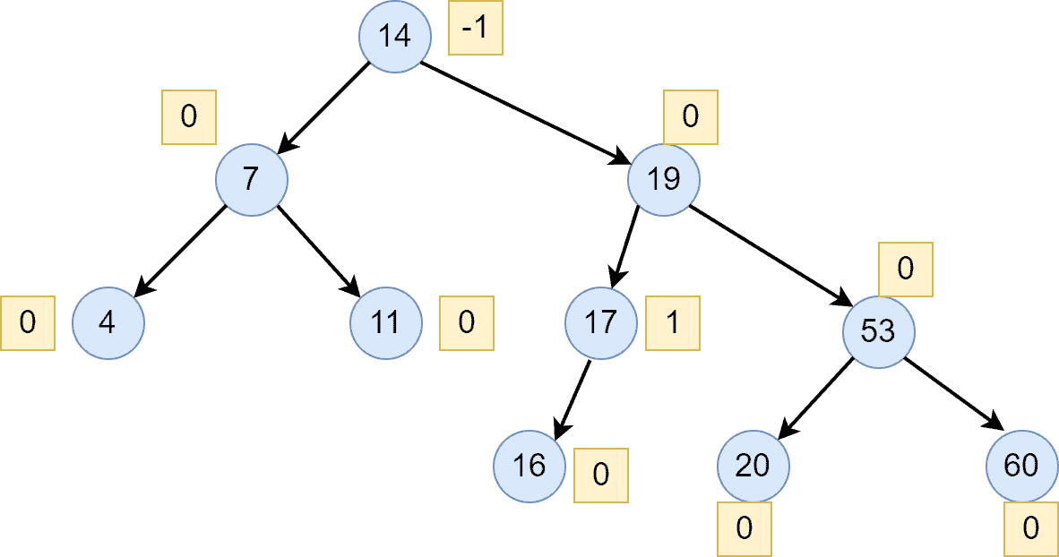
The AVL tree is balanced. Finally, let’s insert the last node with key-value  :
:
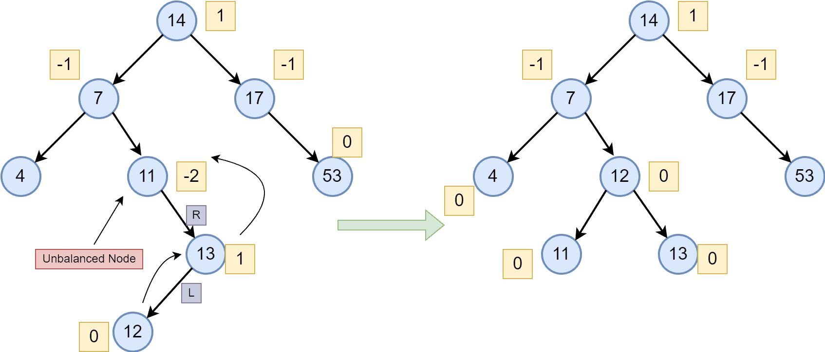
After inserting the node with a value of , the AVL tree becomes unbalanced. Therefore, we first performed a left rotation followed by a right rotation to balance the AVL tree.
Deletion operation in the AVL tree is similar to the BST deletion. But again, we have to calculate the balance factor for each node after performing a deletion operation. When we want to delete a node, we first traverse the tree to find the location of the node. This process is the same as searching nodes or elements in the AVL tree or BST.
When we locate our required node in the given tree, we simply delete the node. After the deletion of the node, we calculate the balance factor for each node. If the AVL tree is unbalanced, we perform the rotations as per the requirement. The time complexity for deleting any element from the AVL is .
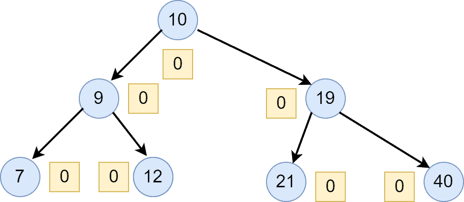
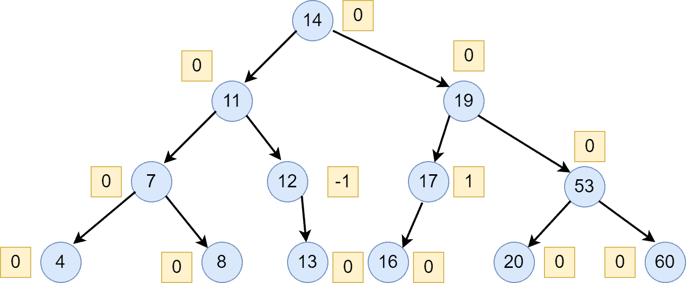
We’re taking an AVL tree to show the deletion example:
Now, for instance, we want to delete the following nodes from the AVL tree:  . Let’s delete node
  first, followed by node :
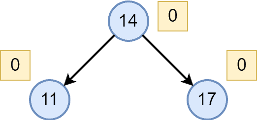
After the deletion of the nodes and , we calculated the balance factor for each node. Additionally, we can see that all nodes are balanced. Hence, we don’t need to perform any rotations here. Let’s delete the next node :
After deleting the node with a value of , we can see that the AVL is not balanced anymore. Therefore, we need to perform a right rotation here in order to balance the AVL tree:
It’s also a self-balancing binary search tree. Therefore, it follows all the prerequisites of a binary search tree. A red-black tree is also known as a roughly height-balanced tree.
There’re two types of nodes in the red-black tree data structure: red and black. Additionally, after performing any tree operations, we may need to apply some rotations and recolor the nodes in order to balance a red-black tree. The complexity of tree operation in the red-black tree data structure is the same as the AVL tree.
The red-black tree is a self-balancing binary search tree with the same complexity as the AVL tree. Therefore, why do we need an additional tree data structure? Let’s discuss.
As we discussed before, we need to apply rotations to balance the tree in the AVL tree. We can often face a situation when we have to perform several rotations. The more the rotations, the more the processing. Hence, the processing would vary based on the number of rotations required. Although, in the red-black tree, there can be a maximum of two rotations required to balance a tree. Hence, the red-black tree is introduced for ease of implementation and execution.
In a red-black tree, each node is color-coded with black or red. The root and leaf nodes are usually colored black. Additionally, if a node is red, its child nodes must be colored black. Let’s look at an RBT tree:
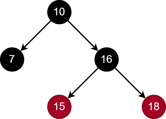
If an RBT has  nodes, the height of RBT can be at most
  . The height of the RBT is a significant property because it makes this tree data structure different from an AVL tree. After every operation, we need to do some rotations and set the color of the nodes as per the current tree. The RBT has the same structure as BST, but it uses an extra bit for storing the color codes of the nodes.
For every node in an RBT, there’re four data: the node’s value, left subtree pointer, right subtree pointer, and a variable to store the color code of the node.
Searching in an RBT is the same as searching any element in the BST. To search any element, we start from the root node and go down to the tree by comparing the key value of the given element. The time complexity of searching any element is .
Insertion operation in the RBT follows some rules of insertion in the BST. If the tree is empty, we need to insert the element and make it black because it would be the root node. When the tree is not empty, we create a new node and color it red.
Additionally, whenever we want to insert any element in the tree, the default color of the new node will always be red. It means the color of the child node and parent node should not be red. We only have to make sure there’re no adjacent red nodes.
After inserting an element, if the parent node of the inserted element is black, we don’t have to do any extra process. It’ll be a balanced RBT. But if the parent of the inserted element is red, we need to check the color of the parent’s sibling node. Hence, we need to check the color of the node, which is at the same level as the parent node.
Deletion operation in RBT is the same as a deletion in the BST. First, we must traverse the tree until the desired node is found. As soon as we locate the node, we remove it from the RBT.
If we delete any red noded, it won’t violate any condition of RBT. Hence, we just need to remove the node like in BST. However, in the case of deleting a black node, it may violate the condition of RBT. Therefore, after we delete any black node, we have to perform some actions like rotations and recoloring in order to rebalance the RBT.
We can find more about the red-black tree and its operations with examples in our introduction to Red-Black Trees.
Let’s now look at the core differences between AVL and Red-Black tree data structure:
| AVL Tree | RBT Tree |
|---|---|
| Strictly height-balanced tree. | Roughly height-balanced tree. |
| Comparatively complex to implement. | Easy to implement. |
| Takes more processing for balancing. | Takes less processing for balancing because a maximum of two rotations are required. |
| Searching operation is faster because of height-balanced structure. | Searching operation is comparatively slow. |
| Insertion and deletion operations are slow. | Insertion and deletion operations are faster. |
| No colour for the nodes. | The nodes can be either red or black. |
| Balance factor is associated with each node. | There’s no balance factor for nodes. |
| Used in databases for faster retrievals. | Used in the language libraries. |
In this tutorial, we discussed AVL and red-black tree data structures. We presented the properties and operations with examples.
Finally, we explored core differences between them.