Binary Tree vs. Binary Search Tree | Baeldung on Computer Science

1. Overview

In this tutorial, we’ll discuss two popular tree data structures: binary tree and binary search tree. We’ll present formal definitions with properties and examples of both tree structures.

Finally, we’ll explain the core conceptual differences between them.

2. Introduction to Binary Trees

A binary tree is a popular and widely used tree data structure. As the name suggests, each node in a binary tree can have at most two children nodes: left and right children. It contains three types of nodes: root, intermediate parent, and leaf node.

A root node is a topmost node in a binary tree. A leaf node can be defined as a node without any children nodes. Finally, excluding the root and leaf nodes, all other nodes are the intermediate parent nodes. Let’s look at an example:

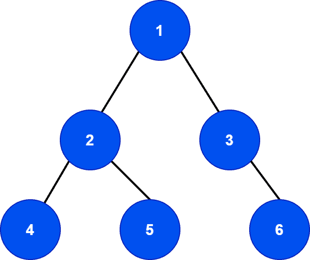
First of all, let’s check if the tree $T_1$ is a binary tree or not. The primary and most important property is that each node can have at most two children nodes. Therefore, we can see that our sample tree $T_1$ obeys this property. Hence, it’s a binary tree.

Here, the node $\mathsf{1}$ is the root node of the binary tree $T_1$ . Moreover, the nodes $4, 5,$ and $6$ are the leaf nodes. Finally, the nodes $2$ and $3$ are the intermediate parent nodes.

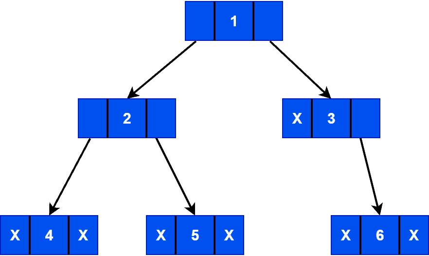
Each node in a binary tree contains three fields: pointer to the left children, data, pointer to the right children. Let’s look at the logical representation of the binary tree $T_1$ :

There’re various types of binary trees. Some of them are the full, perfect, complete, skewed, balanced binary trees. Moreover, the binary tree data structure supports four main operations: searching, insertion, deletion, and traversal.

3. Properties

Let’s discuss some important properties of the binary tree data structure.

There can be a maximum of $\mathbf{(2^{h} -1)}$ nodes in a binary tree with height $\mathbf{h}$ . Let’s take a look at the binary tree $T_1$ . The leaf nodes are at the height of $3$ . Hence, the height of $T_1$ is $\mathsf{3}$ .

Additionally, the height of the root is $\mathsf{1}$ . Hence, the maximum number of nodes with height $\mathsf{1}$ can be $(2^{1} -1) = 1$ . Similarly, the maximum number of nodes $T_1$ can contain would be $(2^{3} -1) = 7$ .

Now given the total number of nodes $N$ in a binary tree, the minimum height or level of the binary tree would be $\mathbf{\lceil Log_{2}(N + 1)\rceil}$ . In $T_1$ , there’re $6$ nodes. Hence, the minimum height or level would be $\lceil Log_{2}(6 + 1)\rceil = 3$ .

We can have a maximum of $\mathbf{2^{L}}$ nodes at the $\mathbf{L}$ level of a binary tree. It can be verified easily. The level of the root node of a binary tree is always $0$ . Hence, there can be a maximum of $2^0 =1$ node, which is valid for all binary trees.

Additionally, a detailed explanation with algorithms on how to calculate the exact number of nodes and level of a binary tree can be found in the tutorial: Number of Nodes in a Binary Tree With Level N.

Let’s assume a binary tree has $L$ leaves. According to the binary tree structure, it should have at least $\mathbf{(|Log_{2}L| + 1)}$ levels. In the case of $T_1$ , we have $3$ leaves. Hence, according to this property, $T_1$ should have at least $(|Log_{2}3| + 1) = 2$ levels which is true.

Now, based on the definition of a binary tree, each node can contain up to two children nodes. Therefore, consider a scenario where all the nodes in a binary tree either contain $2$ or $0$ children. In such a case, the number of nodes with $\mathbf{2}$ children is always one less than the number of nodes with no children.

In $T_1$ , there’re $3$ nodes (nodes with key $4, 5,$ and $6$ ) with no children and $2$ nodes (nodes with key $1,$ and $2$ ) with $2$ children. Hence, this example verifies the property.

4. Introduction to Binary Search Tree

A binary search tree is a sorted tree data structure. Moreover, it follows the properties of the binary tree with some additional properties. Hence, each node can have at most two children nodes. But here, the key of the left subtree is less than the key value of its parent node. Similarly, the key of the right subtree is greater than the key value of its parent node.

Let’s look at an example:

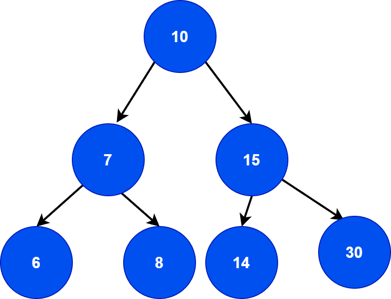
Let’s first determine whether it’s a binary search tree or not. The left children of the root node contain a key that has less value than the key of the root node. Similarly, the right children of the root node contain the key with a greater value than the root node. Finally, the rest of the tree follows both binary tree and binary search tree properties. Hence, we can say that it’s a binary search tree.

Let’s look at another example:

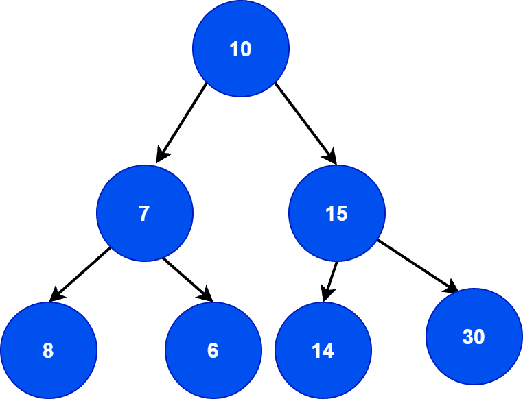
Here, the tree is a binary tree as the root and intermediate parent nodes contain $2$ children nodes each. Although, it’s not a binary search tree. If we look at the leaf nodes of the left subtree, we can observe that it violates the property of the binary search tree. Hence, it’s a binary tree but not a binary search tree.

A more detailed discussion on binary search tree data structure and possible tree operations can be found in the tutorial: A Quick Guide to Binary Search Trees.

5. Differences

There’re similarities between a binary search tree and a binary tree. Both are tree data structures, and each node in both structures can contain at most two children nodes. Regardless of the similarities, they have some core structural and functional differences. Let’s discuss the key differences between them:

6. Conclusion

In this tutorial, we discussed two tree data structures: binary tree and binary search tree. We explained both data structures with examples and presented key differences between them.

Full Archive

About Baeldung

Core Concepts

Operating Systems

Artificial Intelligence

Graph Theory

Latex