Bitonic Sort | Baeldung on Computer Science

1. Introduction

In this tutorial, we’ll study the Bitonic Sort algorithm. Just like the odd-even transposition sort, Bitonic Sort is also a comparison-based sorting algorithm we can easily parallelize.

2. Problem Statement

Let’s say we have an unsorted array $arr$ . We want $arr$ to be sorted in monotonically non-decreasing order. For instance, if we have $arr=[200, 20, 191, 345, 10001]$ at the input, we want to get the output $arr=[20, 191, 200, 345, 10001]$ after sorting.

3. Bitonic Sort

A bitonic sequence is the key concept of the bitonic sort. So, let’s start by defining it.

3.1. Bitonic Sequence

A sequence of $n$ elements $x_{0}, x_{1}, \ldots, x_{n-2}, x_{n-1}$ is called a bitonic sequence if it fulfils either of the following two conditions:

There’s an index $i$ such that $x_{0}, x_1, \ldots, x_i$ is monotonically non-decreasing, and $x_i, x_{i+1}, \ldots, x_n$ is monotonically non-increasing
We can cyclically shift the sequence so that it satisfies the above condition

For instance, the array $[1, 11, 23, 45, 36, 31, 20, 8]$ is a bitonic sequence. Its monotonicity changes at 45: $1 \leq 11 \leq 23 \leq 45$ and $45 \geq 36 \geq 31 \geq 20 \geq 8]$ .

For Bitonic Sort to work effectively, the number of elements in the input array needs to be a power of two. If that isn’t the case, we can extend the array with $2^{\lceil \log_2 n\rceil} - n$ elements larger than those in it. That way, we can make the number of elements of $arr$ a power of two. After sorting, we output the first $n$ elements since all the additional ones are larger.

3.2. General Idea

This algorithm essentially runs two procedures. First, it recursively converts the input array to a bitonic sequence. Then, it merges the two monotonic halves in a way that sorts the entire array:

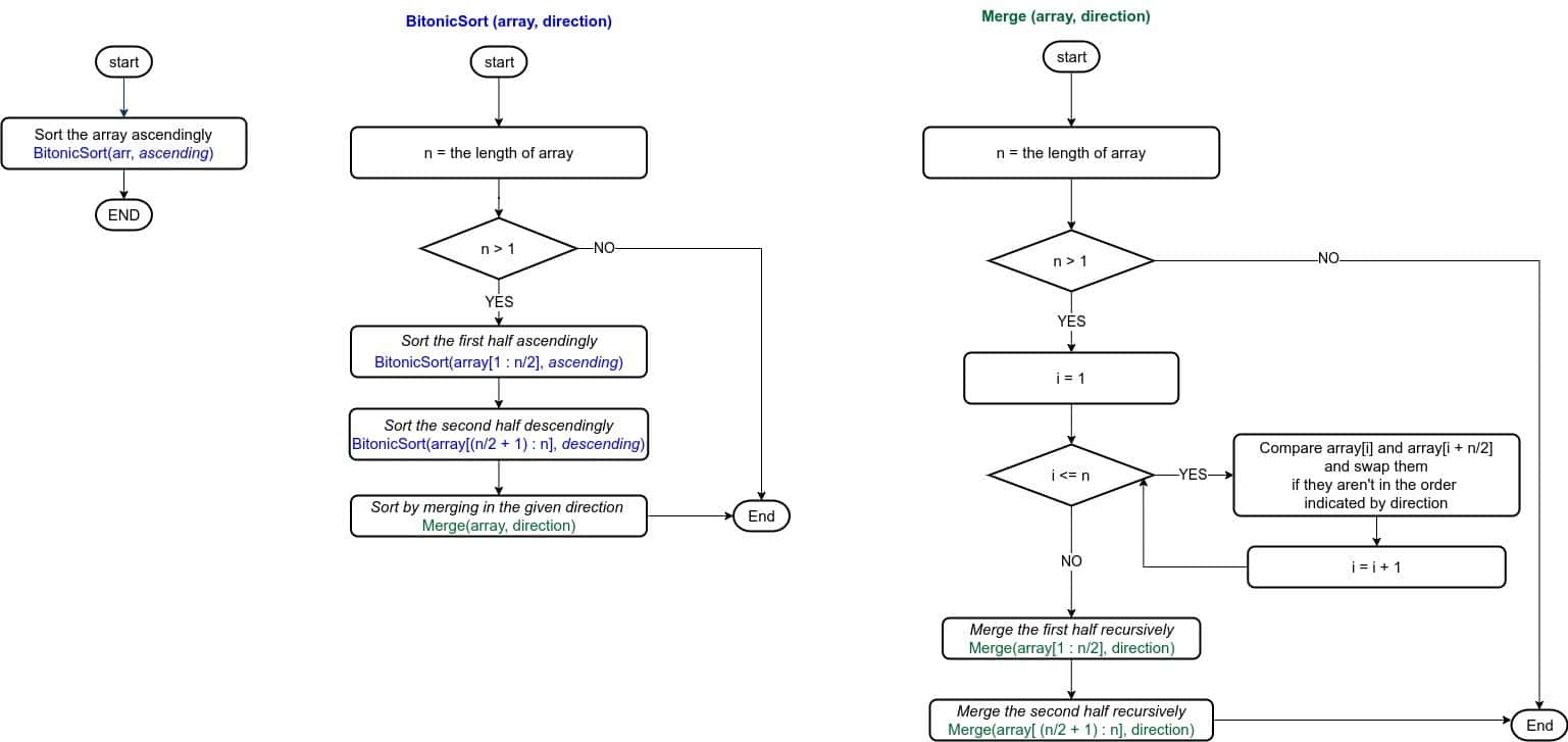
The base case of the first procedure, BitonicSort, is when there’s only one element in $arr$ . As per the definition, single-element arrays are bitonic. The variable $dir$ shows whether the subsequence at hand should be ascending or descending.

The second procedure is Merge. In it, we compare the first element of the first half with the first element of the second half, then the second element of the first half with the second element of the second half, and so on. We swap the elements if the one from the second half is smaller. This results in two subsequences with length $\frac{n}{2}$ such that all the elements in the first one are smaller than all the elements in the second one. We apply these steps recursively to both halves.

3.3. Pseudocode

Now, let’s look into the pseudocode of Bitonic Sort:

The algorithm takes as input an unsorted array $arr$ . We’ll assume that $n$ is a power of 2 since we can always extend the array as explained above. The variable $direction$ stores the sorting direction. Initially, we set it to $ascending$ .

4. Example

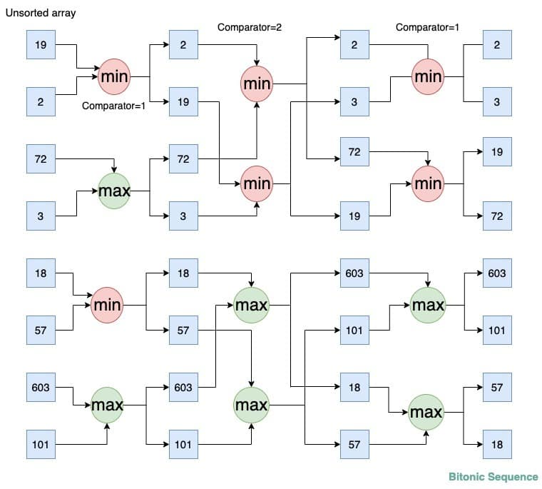
Let’s say the input array is $arr=[19, 2, 72, 3, 18, 57, 603, 101]$ .

4.1. From Unsorted to Bitonic

The following figure shows the execution until the entire array becomes a bitonic sequence with two halves of opposite monotonicities:

As the name suggests, the $min(a, b)$ function sorts and stores $a$ and $b$ in the ascending order whereas the $max(a, b)$ function sorts and stores them in the descending order. The variable $comparator$ denotes the number of elements to skip from the current elements for comparison.

In the first step, we form two 4-element bitonic sequences. First, we apply $min$ to the first two elements, and $max$ to the next two. We then concatenate the two pairs to form a 4-element bitonic sequence: [2, 19, 72, 3]. Afterward, we do the same with the last four elements and get another 4-element bitonic sequence: [18, 57, 603, 101]. Then, we merge monotonic halves to get two ascending and descending sequences: [2, 3, 19, 72] and [603, 101, 57, 18].

4.2. From Bitonic to Monotone

We did $\log 8=3$ steps to get our bitonic sequence. Now, we move to sort it.

Here, we show the complete bitonic sort from the above generated bitonic sequence:

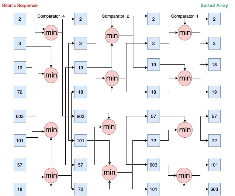
The procedure that sorts the array, in the end, is Merge. In essence, we apply $\boldsymbol{min}$ to elements with closer and closer indices until the entire sequence is sorted.

We start with an 8-element bitonic sequence and sort it recursively to get eight 1-element bitonic sequences. We set $comparator=\frac{8}{2}=4$ . Then, we apply $min$ on the 1^st and 5^th elements (2 and 603), then again on the 2^nd and 6^th elements (3 and 101), and so on until we do it for the 6^th and 8^th elements ( 72, 18). After this step, we get two 4-element subsequences such that all elements of the first one ([2, 3, 19, 18]) are smaller than all elements of the second one ([603, 101, 57, 72]).

Now, we repeat the above process for both halves recursively. We set $comparator=\frac{4}{2}=2$ and apply $min$ on 1^st element and 3^rdelement (2, 19), then again on 2^nd element and 4^th element (3, 18) and finally get: [2, 3, 19, 18]. We do the same for other sequences and get [57, 72, 603, 101].

Lastly, we repeat the above process for each of these four 2-element subsequences to get: [2, 3, 18, 19, 57, 72, 101, 603]. Since the entire array is now sorted, we stop.

5. Time Complexity

There are $\log_2 n$ levels in the recursion tree of $BitonicSort$ since each call halves the input size.

$Merge$ takes $\frac{n}{2}\log_2 n$ comparisons. First, it compares $n/2$ pairs, then $n/4$ pairs in one and $n/4$ pairs in the other subsequence, and so on:

$\frac{n}{2} + 2 \times \frac{n}{4} + 4 \times \frac{n}{8} + \ldots + \frac{n}{2} \times 1 = \frac{n}{2}\times \log_2 n$

From there, the time complexity of Bitonic Sort is $O\left( n (\log n)^2 \right)$ .

6. Scope for Parallelization

Bitonic sort is a sequential sorting algorithm that is inefficient when sorting large volumes of data. But, when performed in parallel, it performs much better.

Parallel processing works by dividing data among processors and processing each chunk at the same time. When all the processors complete their jobs, we combine their partial outputs to produce the final result. So, this way, we can reduce the time needed to do all the steps.

Here, due to the predefined sequence of comparison sequence, the comparisons are independent of the data that is to be sorted. Additionally, the load balancing features help maintain equal load among all the processors.

The parallel version, when we run it on $\boldsymbol{p}$ processors, sorts an $\boldsymbol{n}$ -element array in $\boldsymbol{\theta(\frac{n}{p} (\log n)^2)}$ time.

7. Advantages of Bitonic Sort

Even though the number of comparisons done by bitonic sort is greater than those of other, more popular sorting algorithms such as QuickSort, Bitonic Sort works better in parallel implementations.

The reason is that it always compares input elements in a predefined way that doesn’t depend on the actual input. Thus, we get the best results when we run it on a system with a parallel processor array or on a mesh-based hardware system.

8. Conclusion

In this article, we have studied the Bitonic Sort algorithm. It sorts an array by creating bitonic sequences and reducing the problem size to half at each step. It can run very fast as a parallel algorithm on a multiprocessor system.

Full Archive

About Baeldung

Core Concepts

Operating Systems

Artificial Intelligence

Graph Theory

Latex