Odd-Even Transposition Sort

1. Introduction

In this tutorial, we’ll study the Odd-Even Transposition Sort algorithm. It’s a variant of the classical Bubble Sort, a comparison-based sorting method.

The Odd-Even Transposition Sort was originally developed for running on a multi-processor system, although we can run it on a single processor as well. We also refer to it by the names of Brick Sort and Parity Sort.

2. Odd-Even Transposition Sort Algorithm

In a sorting problem, we are given an unsorted array . We want to be sorted in monotonically non-decreasing order. For instance, if we are given at the input, we want to get the output after sorting.

The Odd-Even Transposition Sort performs the same as the classical Bubble Sort when we run it on a uniprocessor system. However, we harness its full power when running it as a parallel algorithm on a multiprocessor system.

2.1. General Idea

The algorithm follows the divide-and-conquer methodology. The underlying idea is that we process the given array by iterating two phases. We call them the odd phase and the even phase.

In the odd phase, we compare all the odd-indexed elements with their immediate successors in the array and swap them if they’re out of order. In the even phase, we repeat this process for all even-indexed elements and their successors. Then, we iterate over these two phases until we find no more elements to swap. At that point, we exit the algorithm since the array is sorted.

2.2. Pseudocode

Here’s the pseudocode of the odd-even transposition sort:

The algorithm takes as input an unsorted array and the number of elements in it. It uses a variable to denote if is sorted. In the beginning, is since we don’t know if is sorted.

In each iteration of the loop, the algorithm executes odd and even phases.  If it performs no swaps, it sets to and exits the loop.

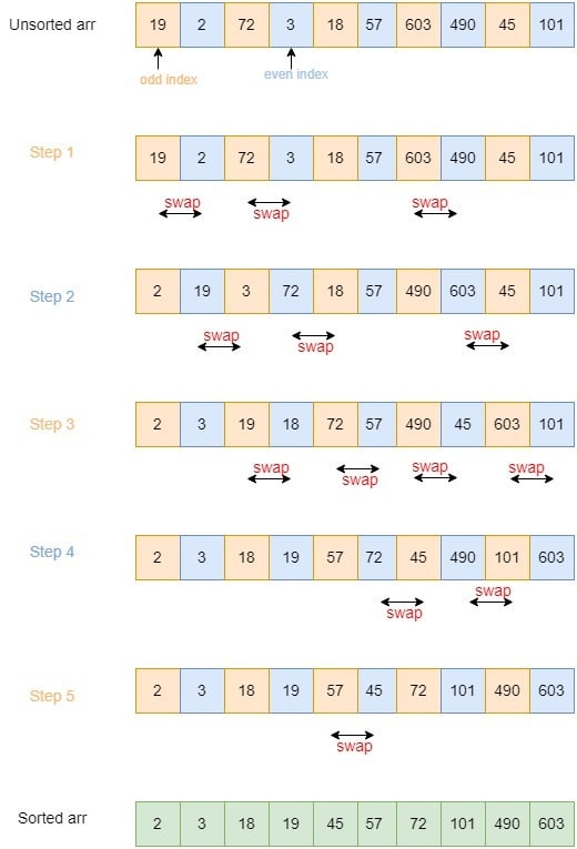
2.3. Example

Let’s say the given array is . It has elements.

In the first step, we execute the odd phase. So, we sort all the pairs that start at the odd positions. Thus, we swap 19 and 2, 72 and 3, and 603 and 490. Having done so, we get .

In the second step, we execute the even phase wherein, we sort all the pairs starting at the even positions. In particular, we swap 19 and 3, 72 and 18, and 603 and 45. At this point, we have .

We repeat odd and even phases at subsequent steps until we sort the entire array:

3. Space and Time Complexity

In this section, let’s discuss the space and time complexity of this algorithm for the uniprocessor case.

On a single processor, the algorithm’s time complexity is because we make comparisons for each of the elements.

This algorithm’s space complexity is . The space complexity in terms of auxiliary storage is because the odd-even transposition sort algorithm is an in-place sorting algorithm. Apart from the space for the input array, it requires only a single temporary variable for swapping the elements and another one for iterating over the array.

4. Scope for Parallelization

A sequential algorithm such as this one may be inefficient when sorting large volumes of data. But, when performed in parallel, it can run fast.

A parallel algorithm runs on multiple processors or cores at the same time and then combines the partial outputs to produce the final result.

The odd-even transposition sort algorithm can be executed on a machine with processors. In such a scenario, each processor takes as input a sub-array containing successive elements of the input. Then, the sub-arrays get sorted in parallel. Afterward, we merge all these smaller sorted sub-arrays to get the final sorted array.

5. Conclusion

In this article, we have studied a variant of Bubble Sort called Odd-Even Transposition Sort.

It offers the same efficiency as Bubble Sort when run on a uniprocessor system. But, it is more efficient when we execute it in parallel.