Finding a Cycle in a Singly Linked-List | Baeldung on Computer Science

1. Overview

In this tutorial, we’ll discuss the problem of finding a cycle in a singly linked list and the starting point of this cycle.

First, we’ll explain the general idea of the problem and then discuss two approaches to solving it. Secondly, we’ll present two exceptional cases and see how can one of the approaches be updated to handle them.

In the end, we’ll present a comparison between all the provided approaches.

2. Defining the Problem

Suppose we have a linked list $A$ , which has $n$ nodes. We want to check if the list is cyclic or not. Also, we want to find the beginning of this cycle, if found.

Before we start with the solutions, we need to know what the cycle in a list means.

As we know, the list is a collection of nodes in which each node contains a reference (in other words, a link) to the next node. We say that the list is cyclic when the last node points to one of the nodes in the list

Let’s check the example for better understanding:

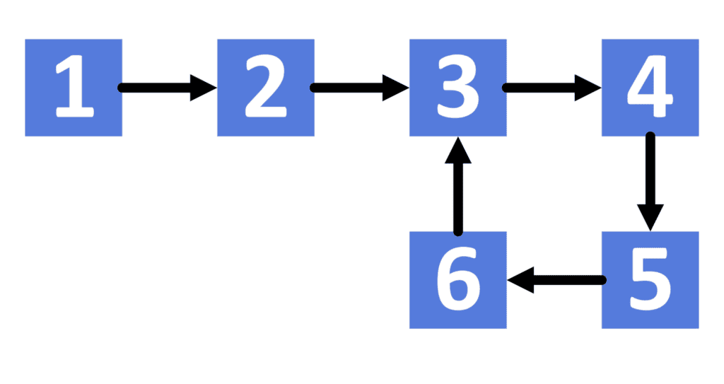
Note that we can have only one cycle inside a list. Besides, the cause of the cycle will always be that the last node is pointing to a node inside the list because each node points to exactly one node.

3. Visited Approach

3.1. General Idea

In the simple list with no cycles, we can iterate over its elements using $while$ loop as follows:

algorithm iterateList(A):
    // INPUT
    //   A = The linked list

    iter <- A.head
    while iter != null:
        // ...
        iter <- iter.next

The reason is that, since we don’t have a cycle, the last element points to $null$ . Take a look at the example that shows an acyclic list:

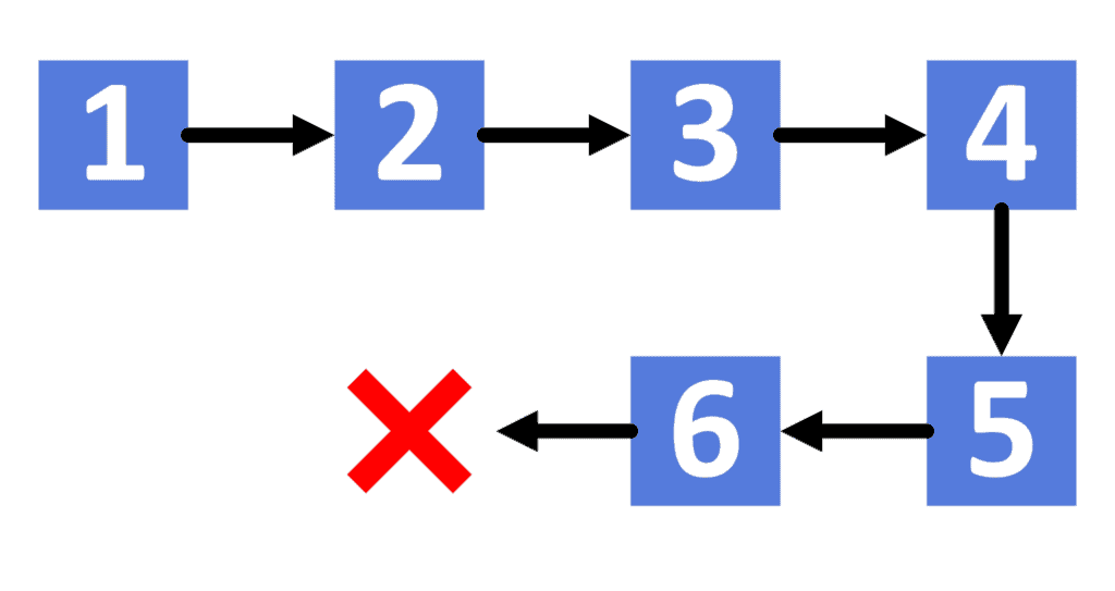
However, when we have a cycle, we can’t iterate using the same way. The reason is that the last node points to another one. Therefore, the algorithm will enter an infinite loop.

To solve this issue, we can add a variable to each node that tells us whether we’ve visited it before or not. Let’s call it $\boldsymbol{visited}$ .

3.2. Implementation

Take a look at the implementation of the visited approach:

algorithm findCycleVisited(A):
    // INPUT
    //   A = The linked list
    // OUTPUT
    //   Returns the starting node of the cycle if it exists, or null otherwise

    answer <- null
    node <- A.head

    while node != null:
        if node.visited = true:
            answer <- node
            break
        node.visited <- true
        node <- node.next

    node <- A.head
    while node != null:
        if not node.visited:
            break
        node.visited <- false
        node <- node.next

    return answer

The implementation consists of two main steps.

In the first step, we check whether there is a cycle in $A$ . At first, we initialize $answer$ by $null$ . This is so that if we can’t find any loop, the $answer$ remains $null$ .

Next, we iterate over the nodes in $A$ using the iterator $node$ . In each step, we check whether we visited the current node before. If so, it means we reached a cycle, and the current node is the starting point. Therefore, we store $node$ inside $answer$ and stop the loop.

In case we haven’t visited this node before, we mark it as visited and continue to the next element.

Once we’re done with the first step, we mark all nodes as unvisited to restore the list to its original state. This is to allow us to use this variable in other algorithms.

Finally, we return the resulting $answer$ .

The complexity of the visited approach is $\boldsymbol{O(n)}$ , where $n$ is the length of the list.

4. Special Cases for the Visited Approach

In some problems or program language, it’s tough to edit the structure of the nodes. As a result, we might not be able to add the $visited$ variable. However, we might have a unique variable for each element. Let’s call it $id$ .

4.1. Small Integer IDs

In case $\boldsymbol{id}$ is an integer in the range $\boldsymbol{[0, MaxVal]}$ , where $\boldsymbol{MaxVal}$ is relatively small, we can add a new boolean array with $\boldsymbol{MaxVal+1}$ elements. In each step, we check the value of $\boldsymbol{visited[node.id]}$ , rather than checking the value inside the element.

Let’s take a look at the implementation:

algorithm findCycleSmallIntegers(A):
    // INPUT
    //   A = The linked list
    // OUTPUT
    //   Returns the starting node of the cycle if it exists, or null otherwise

    answer <- null
    node <- A.head
    visited <- array of false values

    while node != null:
        if visited[node.id] = true:
            answer <- node
            break
        visited[node.id] <- true
        node <- node.next

    return answer

Firstly, we initialize $answer$ with $null$ , which will hold the resulting answer. Also, we’ll initialize the array $visited$ with false values.

Secondly, we’ll iterate over $A$ . For each node, we check whether we’ve visited it before or not. To do this, we use the $visited$ array.

If we haven’t visited it before, we assign $true$ to its location inside $visited$ and move to the next. Otherwise, we update $answer$ and break the loop.

Finally, we return the resulting $answer$ .

Note that if we have negative values, such that the id’s range is $[-a,+b]$ , we can still use this approach after shifting all values by $a$ . Hence, the id’s range will be $[0,a+b]$ and the position of id $x$ will be $x+a$ .

The complexity of this approach is $\boldsymbol{O(n+MaxVal)}$ , where $n$ is the size of the list, and $MaxVal$ is the maximum value of the ids.

4.2. TreeSet Approach

In case the $id$ is not an integer or has a relatively large value, we can’t use an array. Thus, we solve this case by using either a TreeSet or a HashSet data structure. In this tutorial, we’ll use a TreeSet to store the visited elements.

Let’s take a look at the implementation:

algorithm findCycleTreeSet(A):
    // INPUT
    //   A = The linked list
    // OUTPUT
    //   Returns the starting node of the cycle if it exists, or null otherwise

    answer <- null
    node <- A.head
    set <- empty TreeSet

    while node != null:
        if set.contains(node.id):
            answer <- node
            break
        set.add(node.id)
        node <- node.next

    return answer

Similarly to the previous approach, we initialize $answer$ with $null$ , which will hold the resulting answer. Besides that, we define $set$ as a new empty TreeSet that will hold the visited ids.

Same as before, we’ll use the iterator $node$ to iterate over $A$ . However, in this approach, we’ll use the $\boldsymbol{set}$ data structure to check whether we reach a visited node.

If we don’t find the $id$ inside the $set$ , we move to the next element and add it to $set$ . Otherwise, we update the $answer$ and break the loop.

Finally, we return the $answer$ .

The complexity of this approach is $\boldsymbol{O(n \times log(n))}$ , where $n$ is the number of elements.

5. Two-Pointers Approach

In this section, we’ll explain a different idea to finding a cycle in a list.

5.1. General Idea

First of all, let’s define two iterators $node1$ and $node2$ initializing them with $A.head$ .

Next, we iterate over $\boldsymbol{A}$ . Each time, we move $\boldsymbol{node1}$ one step, while we move $\boldsymbol{node2}$ two steps. We continue this process until we either reach $\boldsymbol{null}$ or $\boldsymbol{node1}$ becomes eqaul to $\boldsymbol{node2}$ .

If we reach $null$ , we declare that no cycle is found. On the other hand, if $node1$ becomes equal to $node2$ , then we reached a loop and $node1$ points to one of its nodes.

To find the start of the cycle, we must find the size of the loop first. We can do this by moving $node1$ only until it becomes equal to $node2$ again and counting the steps. Hence, we get the size of the cycle denoted as $m$ .

Now, let’s start $\boldsymbol{node1}$ from the beginning of $\boldsymbol{A}$ , and $\boldsymbol{node2}$ from the $\boldsymbol{m^{th}}$ node. We keep moving $\boldsymbol{node1}$ and $\boldsymbol{node2}$ one step until they meet. At this point we can either return $node1$ or $node2$ as the beginning of the cycle.

5.2. Implementation

Let’s check the implementation:

algorithm findCycleTwoPointers(A):
    // INPUT
    //   A = The linked list
    // OUTPUT
    //   Returns the starting node of the cycle if it exists, or null otherwise

    answer <- null
    node1 <- A.head
    node2 <- A.head
    foundLoop <- false

    while node1 != null and node2 != null and node2.next != null:
        if node1 = node2:
            foundLoop <- true
            break
        node1 <- node1.next
        node2 <- node2.next.next

    if not foundLoop:
        return null

    m <- 1
    node1 <- node1.next
    while node1 != node2:
        node1 <- node1.next
        m <- m + 1

    node1 <- A.head
    node2 <- A.head
    for j <- 1 to m:
        node2 <- node2.next

    while node1 != node2:
        node1 <- node1.next
        node2 <- node2.next

    return node1

We can split this implementation into four parts:

We check whether we have a cycle or not. This is done by moving $node1$ one step, and $node2$ two steps each time. The process continues until they meet. When they meet, we declare finding a cycle. After the loop ends, we check whether we found a loop. If so, we return $null$ and terminate the algorithm.
We calculate the size of the cycle of $m$ . We move $node1$ until it meets with $node2$ again. Note that we move the $node1$ one time before the loop because, at first, they are equal.
Assign $A.head$ to $node1$ and move $node2$ until it points to the $m^{th}$ node.
Move $node1$ and $node2$ together until they meet. Once they meet, return any of them.

The complexity of this approach is $\boldsymbol{O(n)}$ , where $n$ is the size of the list. Let’s explain the reason behind the linear complexity.

5.3. Two-Iterators Proof of Concept

First of all, let’s explain the idea behind the two iterators. Since $node2$ is moving twice as fast as $node1$ , then once $node2$ will be the first one to enter the cycle. After this, $node1$ will enter the cycle.

At this point, we can be sure that $\boldsymbol{node2}$ will catch up to $\boldsymbol{node1}$ , after at most $\boldsymbol{m}$ steps, because it’s moving faster. Before this happens, we have multiple cases:

If they meet, we must have a cycle because $node2$ came back to meet $node1$ .
If $\boldsymbol{node2}$ is one step before $\boldsymbol{node1}$ , then in the next step they will meet. Hence, we have a cycle.
In case $node2$ is two steps before $node1$ , then in the next step, $node2$ will be one step before $node1$ , which is similar to case 2.

In general, since $\boldsymbol{node2}$ moves two steps forward, the distance between both iterators will reduce by one step each time until they finally meet.

As a result, we can conclude that if we have a cycle, then $node2$ will catch up to $node1$ , and they’ll meet at the same location after no more than $n$ steps.

5.4. Cycle Starting Node Proof of Concept

To get the beginning of the cycle, we started $node1$ from the beginning of $A$ and $node2$ from the $m^{th}$ node. Let’s prove that they must meet after no more than $n$ steps.

First of all, let’s define the distance as the number of steps needed for $node1$ to reach $node2$ . In the beginning, the distance equals $m$ , which is the size of the cycle.

Since both iterators move at the same speed, this distance will remain the same. Also, $\boldsymbol{node2}$ will be the first to enter the cycle, followed by $\boldsymbol{node1}$ after $\boldsymbol{m}$ steps. When this happens, suppose $\boldsymbol{node1}$ still needs $\boldsymbol{m}$ steps to reach $\boldsymbol{node2}$ .

However, since both of them are inside the cycle, if $\boldsymbol{node1}$ moves $\boldsymbol{m}$ steps forward, it’ll reach its current location. The reason is that the cycle has $m$ elements. So, moving $m$ steps from a node will get us back to the same node.

As a result, the only way that $node2$ is still in front of $node1$ by $m$ steps is if they’re at the same node. Hence, this node is the starting node. Also, $node1$ needs at most $n$ steps to reach the beginning of the cycle.

6. Comparison

Take a look at the differences between previous approaches:

	Visited Approach	Small Integer Ids Approach	TreeSet Approach	Two-Pointers Approach
Time Complexity	$O(n)$	$O(n+MaxVal)$	$O(n \times log(n))$	$O(n)$
Memory Complexity	$O(n)$	$O(n+MaxVal)$	$O(n)$	$O(1)$
Use Cases	Only when we can edit the structure of nodes	Only when the ids are relatively small integers	General approach	General approach

By memory complexity, we mean the additional needed memory regardless of the memory already occupied by the list.

As we can see, the visited approach is simpler to implement and easier to understand. But, to use it, we need to add the $visited$ variable to the nodes of the linked list. Hence, the $O(n)$ memory complexity.

On the other hand, when we have small integer ids inside the list, it’s better to use the small integers approach.

Regarding the TreeSet approach, its complexity is bigger than other approaches. Thus, it’s usually not the best one to go with.

A two-pointers approach is a general approach that can handle any case. Therefore, we can always use it.

Nevertheless, it takes a little more time than the visited approach because we iterate over each element about six times.

7. Conclusion

In this tutorial, we discussed finding a cycle in a singly linked list and the starting point of this cycle.

Firstly, we explained the general idea of the problem and discussed two approaches that solve it. Besides that, we presented two special cases related to the first one.

In the end, we showed a comparison between all the approaches in terms of time and memory complexity. Also, we discussed the best practices for using each of them.

Core Concepts

Operating Systems

Artificial Intelligence

Graph Theory

Latex

Full Archive

About Baeldung