Binomial Heaps | Baeldung on Computer Science

1. Introduction

In this tutorial, we’ll study binomial heaps. We use them to implement priority queues and discrete-event simulation for queuing systems.

2. Binomial Tree

A binomial heap is based on a binomial tree. So first, we’ll briefly introduce binomial trees.

2.1. Definition

Formally, we can define a binomial tree $B_k$ of order $k$ recursively:

For $k=0$ , $B_{0}$ contains only the root node $R$ .
For $k>0$ , the root $R$ of $B_{k}$ has roots of $B_{0}, B_{1}, \ldots, B_{k-1}$ as its children. So, $B_k$ contains root $R$ and $k$ binomial subtrees.

The root of the binomial tree $B_{k}$ has $k$ children (i.e., its degree is $k$ ), where the $i^{th}$ child ( $i=1,2,\ldots,k$ ) is again a binomial tree of order $k-i$ :

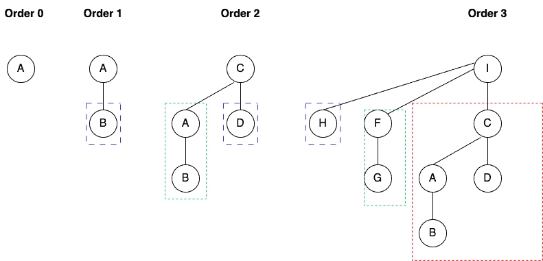
As we see, it’s a recursive and ordered data structure.

A binomial tree $T$ of order $k$ has $2^k$ nodes, and its height is $k$ .

3. Binomial Heap

We define a binomial heap as a set of binomial trees satisfying the min-heap property.

That means that the value of each node is the minimum of the values in its sub-tree.

Further, we link root nodes of the binomial trees in the binomial heap to get a linked list $L_{H}$ .

3.1. Formal Definition

Formally, a binomial heap $H$ is a collection of binomial trees $B_k$ such that:

Each binomial tree $B_{k}$ in $H$ has the min-heap property (is heap-ordered).
For each $k=0,1,2,\ldots$ , $H$ contains at most one binomial tree of order $k$ .

The first property tells us the minimal elements of the trees are in the linked list. The second property tells us that a binomial heap $\boldsymbol{H}$ with $\boldsymbol{n}$ nodes has $\lfloor \log n \rfloor + 1$ binomial trees.

3.2. Example

Let’s check out an example:

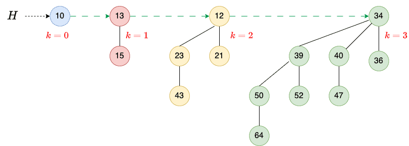
Here, the heap $H$ (15 nodes) consists of four binomial trees: $B_{0}$ (1 node), $B_{1}$ (2 nodes), $B_{2}$ (4 nodes), and $B_{3}$ (8 nodes).

Each binomial tree is heap-ordered, and the trees’ orders are unique. We can also see a linked list containing the root nodes in the increasing order of their degrees.

4. Operations

Let’s learn the basic operations we can perform on a binomial heap:

Create a new binomial heap
Find the minimum key
Merge two heaps
Insert a key

A binomial heap has other interesting operations, e.g., deleting a node, extracting a node with a minimum key, and changing the key of a particular node. However, we won’t cover them in this tutorial.

4.1. The Node Data Structure

We can represent each node $x$ in the binomial heap $H$ with the following data structure:

a variable KEY to store the node’s content (key)
a pointer PARENT to hold the link to its parent
a pointer CHILD to keep the link to its leftmost child
a pointer SIBLING to the leftmost child’s first right sibling
an integer DEGREE to store its degree

We can implement the heap without PARENT and DEGREE, but they make the algorithms for the operations easier to understand and formulate.

Additionally, we’ll use HEAD to point to the leftmost binomial tree of the heap $H$ . Each node in the binomial tree in a heap keeps track of all its children. For instance:

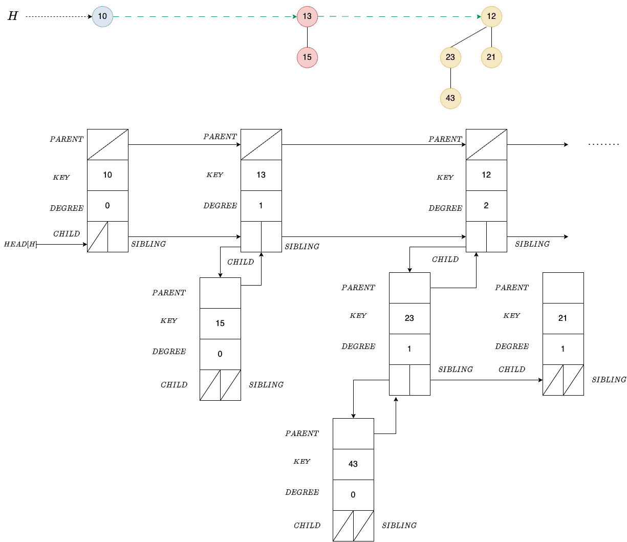
The parent pointers of the root and child and sibling pointers of the leaves are empty. The sibling pointer of a root points to the next tree’s root.

4.2. Make an Empty Heap

To create an empty heap, we allocate the memory for the head node and set the pointers to empty values (usually denoted as $\varnothing$ , NIL, or NULL in textbooks).

This is an $O(1)$ operation regarding space and time.

4.3. Find the Minimum Key

We already know that the root of a binomial tree in a binomial heap $H$ contains the tree’s minimum key.

Since the roots are in a linked list, we must traverse it to find the minimum.

This operation’s time complexity is $O(\log n)$ , where $n$ is the total number of nodes in the binomial heap $H$ . This is so because a binomial heap with $n$ nodes has at most $\log_2 n + 1$ trees.

5. Merge Two Heaps

Let $H_1$ and $H_2$ be two binomial heaps with $n_1$ and $n_2$ nodes.

5.1. Merging Two Binomial Trees of the Same Order

We’ll use a helper method of merging two binomial trees of the same degree. The result of merging two trees of order $\boldsymbol{k}$ is a tree of order $\boldsymbol{k+1}$ :

We first compare the root nodes’ keys. To keep the min-heap property, the root with a smaller key should become the parent of the other tree’s root.

Since we use a fixed number of pointers and variables in a node structure, this operation has a constant time complexity $O(1)$ .

5.2. Merging Two Heaps

The idea is to merge the sorted root lists of the input heaps $H_1$ and $H_2$ so that it’s also sorted. We can do that using MergeSort for sorted linked lists. Then, we traverse the list merging the successive pairs of roots with the same degree to make sure the resulting heap has at most one tree of any particular order:

The list $L_H$ is sorted in the non-decreasing order. For any possible degree, it contains at most two roots of that degree. Furthermore, any two roots with the same degree will be next to each other in the list.

In each while loop iteration, we examine the degrees of two neighboring roots ( $current$ and $next$ ) and merge their trees if they’re equal. If so, we store the resulting tree’s root in the place of the left neighbor.

Otherwise, we check if the left neighbor has a greater degree than the right one. This can happen if the degree sequence contains the pattern $k \rightarrow k \rightarrow k+1 \rightarrow k+1$ :

We merge the first two roots to get $k+1 \rightarrow k+1 \rightarrow k+1$
Then, we get $k+2 \rightarrow k+1$
To maintain the order, we switch the roots to get $k+1 \rightarrow k+2$

Without switching, we won’t correctly merge the trees if the first degree after the pattern is $k+2$ . So, for example, we would have $k+2 \rightarrow k+1 \rightarrow k+2$ and miss merging the $k+1$ trees if we don’t switch the first two in the triple.

5.3. Example

Let’s understand the Merge operation with an example. So, we have two heaps:

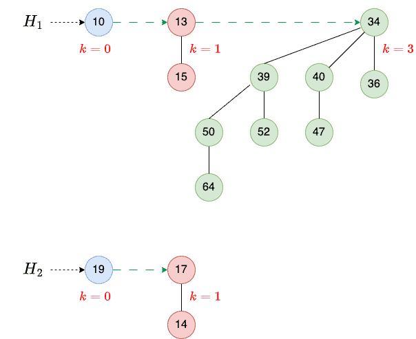
We first look at $H_1$ and $H_2$ to find binomial trees of order 0. We combine them to get a binomial tree of order 1 (step 1). Then, we combine trees of order 1 to get a tree of order 2 (step 2). There’s only one tree of order 3, so we add it to the new heap:

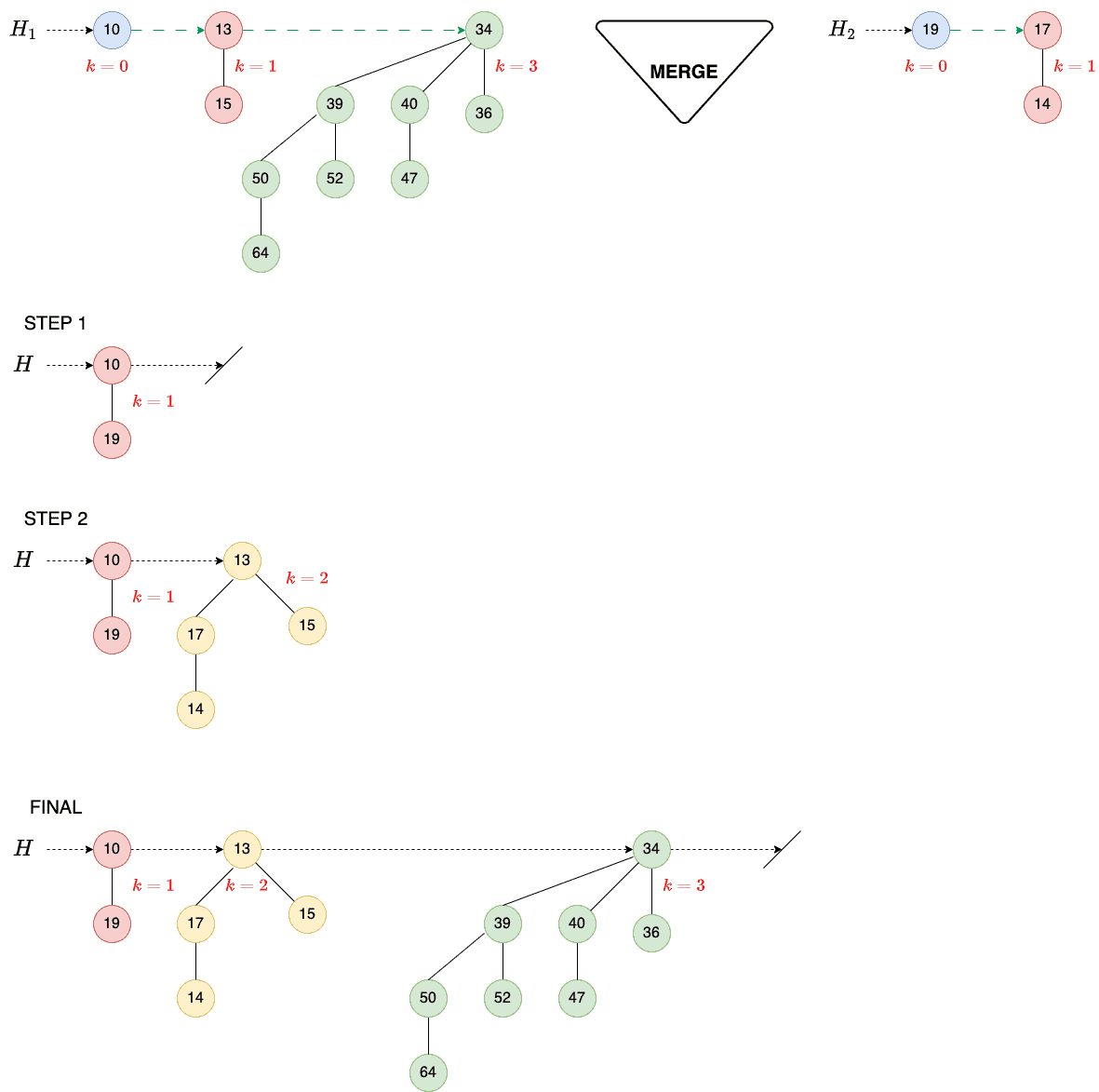
So, our final heap $H$ contains three trees of orders 1, 2, and 3.

5.4. Complexity

Our heaps $H_1$ and $H_2$ have $n_1$ and $n_2$ nodes. The resulting heap $\boldsymbol{H}$ has $\boldsymbol{n_1+n_2}$ nodes.

Now, $H_1$ contains at most $\log_2 n_1 + 1$ trees and $H_2$ contains at most $\log_2 n_2 + 1$ trees, so $H$ will contain at most $\boldsymbol{\log_2 n_1 + \log_2 n_2 + 2}$ trees.

Merging the sorted lists takes $O(\log n_1 + \log n_2)$ time. Since no more than $\log_2 n_1 + \log_2 n_2 + 1$ mergers, switches, and pointer movements are possible, the worst-case time complexity is $\boldsymbol{O(\log n_1 + \log n_2)=O(\log (n_1 + n _2)}$ .

The right-hand side follows from taking the logarithms of:

$(n_1 + n_2)^2 \geq n_1 \times n_2$

6. Insert a Key

To insert a new key $z$ into $H$ , we first initialize a new node ( $x$ ) and set its key to $z$ . Then, we create a one-node binomial heap $H_1$ with $x$ as its root and merge it with $H$ :

We complete the procedure by deleting the temporary binomial heap $H_1$ , i.e., freeing its memory.

6.1. Complexity

This operation’s time and space complexity is governed by the time and space complexity of merging two heaps.

For the insert, we have $n_1=n$ and $n_2$ =1. Thus, its time complexity is $O(\log n)$ , and its space complexity is $O(n)$ .

6.2. Example

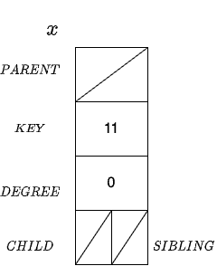
Let’s add a node $x$ with key 11 to our heap $H$ . So, we first assign memory and create node $x$ :

Then, we create an empty heap $H_1$ and set its head to node x:

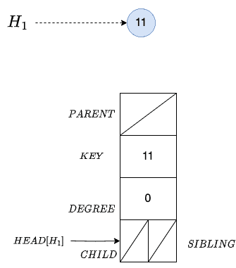
As a result, we now have two heaps, $H$ and $H_1$ :

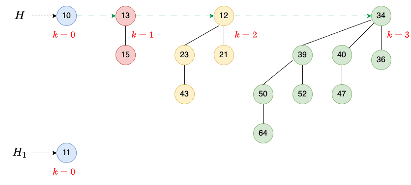
Then, we merge them:

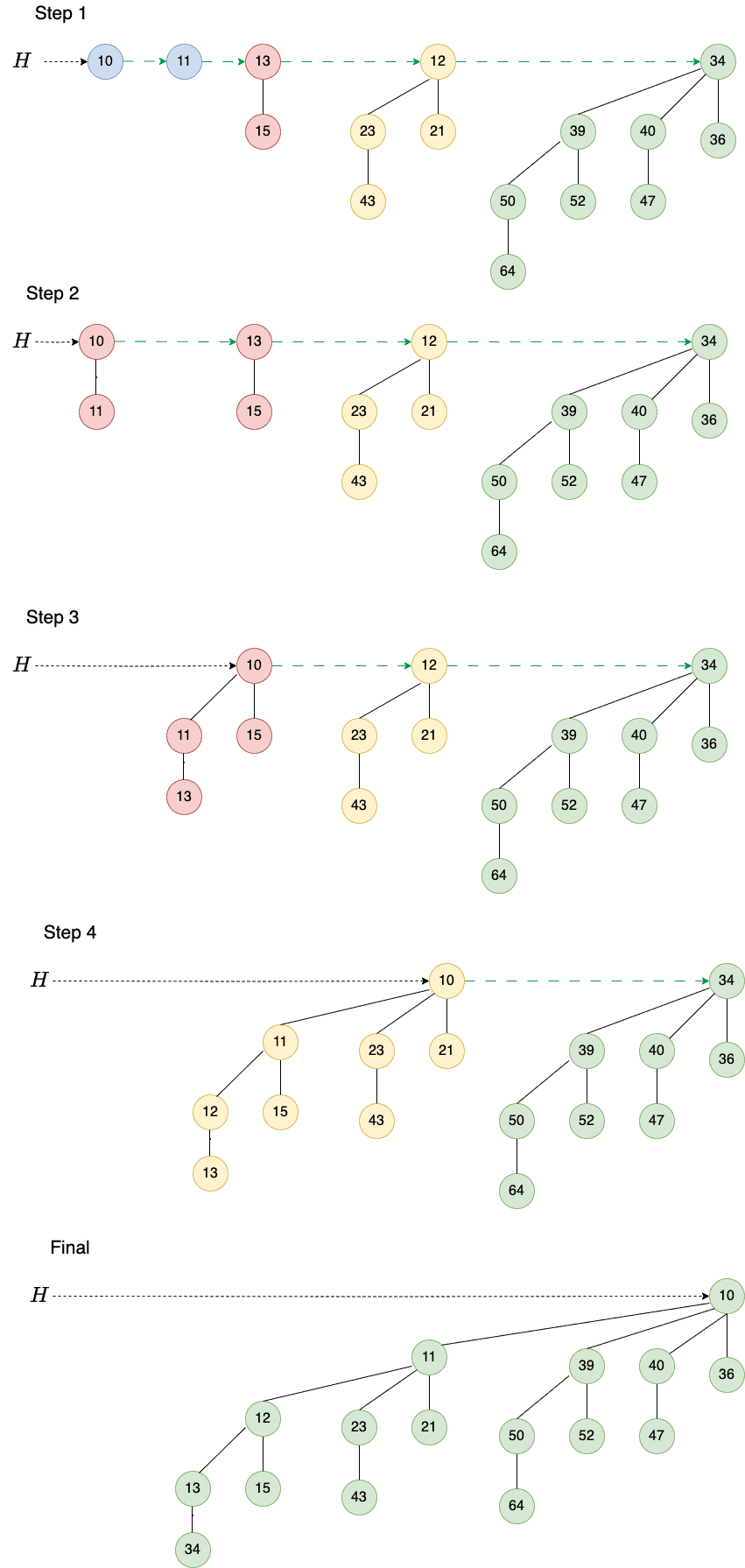
The result is a binomial heap containing a single binomial tree of order 4.

7. Binary Heap vs. Binomial Heap

A binary heap with height $h=\log_2 n$ is a binary tree that can hold any number of elements up to $n$ :

On the other hand, a binomial heap is a collection of smaller binomial trees where the number of elements in a binomial tree of order $k$ is $2^k$ . So, we know the number of nodes in the binomial tree without looking into it.

Further, the merge operation for two binomial heaps $H_1$ with $n_1$ nodes and $H_2$ with $n_2$ nodes has the complexity of $\boldsymbol{O(\log (n_1 + n_2)}$ . This is faster than that of a binary heap ( $\boldsymbol{O(n_1 + n_2)}$ with the same number of nodes).

On the flip side, finding the minimum key in a binary heap is a constant-time operation since the root of a binary heap always contains the minimum key. In contrast, we need to search a list of roots in a binomial heap to find the minimum.

8. Conclusion

In this article, we explained binomial heaps and their properties and studied the operations we can perform on them.

We primarily use binomial heaps to implement priority queues. We merge them more efficiently than binary heaps, although finding the minimum in a binary heap is faster.

Full Archive

About Baeldung

Core Concepts

Operating Systems

Artificial Intelligence

Graph Theory

Latex