

Yes, we're now running our only Summer Sale. All Courses are 30% off until 20th July, 2026:
Intuitive Explanation of the Expectation-Maximization (EM) Technique
Last updated: February 28, 2025
Learn through the super-clean Baeldung Pro experience:
>> Membership and Baeldung Pro.
No ads, dark-mode and 6 months free of IntelliJ Idea Ultimate to start with.
1. Introduction
In this tutorial, we’re going to explore Expectation-Maximization (EM) – a very popular technique for estimating parameters of probabilistic models and also the working horse behind popular algorithms like Hidden Markov Models, Gaussian Mixtures, Kalman Filters, and others. It is beneficial when working with data that is incomplete, has missing data points, or has unobserved latent variables. Therefore it is an excellent addition to every data scientist toolbox.
2. The Likelihood Function
Generally speaking, when estimating the parameters of a given model, we’re searching for the ones that “fit” our data the best. Meaning that if we were to use these exact parameters in our model and then sampled from the model itself, the resulting data should be as close as possible to the real data that we have. To describe this search space, we use a function that takes as an input a combination of parameters  and outputs the probability that we’ll get this sample of data, denoted as
  . This is the likelihood function, and it is described as a conditional probability as follows:
![\[L(\boldsymbol{\theta} ; \mathbf{X})=p(\mathbf{X} \mid \boldsymbol{\theta})\]](/wp-content/ql-cache/quicklatex.com-3955f7eccdc6cb89760bb97bacec0978_l3.svg "Rendered by QuickLaTeX.com")
The natural thing is to try to maximize this function with respect to our parameters so that we can get the best fit. This is known as the method of Maximum Likelihood Estimation. But what if our data has a latent unknown variable  that we cannot observed or formulate? Then the likelihood of our data would be modeled as a joint probability, and we would need to marginalize out the variable and maximize the marginalized likelihood instead:
![\[L(\boldsymbol{\theta} ; \mathbf{X})=p(\mathbf{X} \mid \boldsymbol{\theta})=\int p(\mathbf{X}, \mathbf{Z} \mid \boldsymbol{\theta}) d \mathbf{Z}\]](/wp-content/ql-cache/quicklatex.com-0b70087f4ba83b932444dd42f53f6567_l3.svg "Rendered by QuickLaTeX.com")
This addition to the likelihood function makes it very hard to optimize, and sometimes the equations needed to find the maximum intertwine and cannot be solved directly. But EM overcomes these limitations by iteratively using guesses until we end up with the answer. At first, it might not be apparent why that would work. Still, the EM algorithm is actually guaranteed to converge at a local maximum of our likelihood function, and we’re going to look into how exactly that happens.
3. Intuitive Coin Flipping Example
Let’s first look at a simple coin-flipping example to develop some intuition. We have two coins which we’ll name A and B. Each has some unknown probability of getting heads –  and
and  . Suppose that we want to find what these values are. We can experimentally find them by gathering data. So we take a coin randomly and flip it ten times. And then let’s say we repeat that procedure five times, amounting to 50 coin tosses worth of data:
| Coin | Flips | # coin A heads | # coin B heads |
|---|---|---|---|
| B | HTTTHHTHTH | 0 | 5 |
| A | HHHHTHHHHH | 9 | 0 |
| A | HTHHHHHTHH | 8 | 0 |
| B | HTHTTTHHTT | 0 | 4 |
| A | THHHTHHHTH | 7 | 0 |
Since we denoted each time which coin we were using to take the series of flips, answering would be pretty easy – it’s just the proportion of heads relative to the number of tosses with each coin:
![\[\boldsymbol{\theta_A} = \frac{\text{ \# of heads using coin A }}{\text{total \# of flips using coin A}} = \frac{24}{30}=0.8\]](/wp-content/ql-cache/quicklatex.com-921816ea53a4e1cbdcdbdd201c6a4643_l3.svg "Rendered by QuickLaTeX.com")
![\[\boldsymbol{\theta_B} = \frac{\text{ \# of heads using coin B}}{\text{total \# of flips using coin B}}= \frac{9}{20}=0.45\]](/wp-content/ql-cache/quicklatex.com-57b5d430e1ad91be20efaaa30472d1a2_l3.svg "Rendered by QuickLaTeX.com")
This intuitive solution can be proven to be the maximum likelihood estimate by analytically solving the equations needed to maximize the likelihood function of a Binomial model of the coins here. But what if somehow we lost the data about the identity of each coin we were using throughout the experiment? We’ll end up with data that is incomplete and has one latent variable, which we’ll call – the identity of the coin used.
4. Expectation-Maximization as a Solution
Even though the incomplete information makes things hard for us, the Expectation-Maximization can help us come up with an answer. The technique consists of two steps – the E(Expectation)-step and the M(Maximization)-step, which are repeated multiple times.
Lets’ look at the E-step first. You could say that this part is significantly related to having an educated guess about the missing data. So in our example, can we guess the coin that was used to generate the flips? Well, yes, but it won’t always be the most educated guess, so what can we do?
One thing that would be much better is not to force ourselves to assume one coin or the other, but instead, estimate the probability that each coin is the true coin given the flips we see in the trial. We can then use that to proportionally assign heads and tails counts to each coin. There is a small detail though. In order to estimate that, we would need to know and . So let’s throw a wild guess at them instead, say  and
and  and give it a shot.
For example, imagine we get the outcome HHHHHTTTTT. Given our guess for and , we can use the binomial distribution formula to estimate the probability that we get this exact the series of flips  given each of our coins.
![\[P(E \mid Z_{A})=P(HHHHHHHHT \mid \text{A chosen} )=\left(\begin{array}{l} n \\ x \end{array}\right) \theta_A^{x} (1-\theta_A)^{n-x}\]](/wp-content/ql-cache/quicklatex.com-3b57265094497422592e5e03f58eb69c_l3.svg "Rendered by QuickLaTeX.com")
![\[P(E \mid Z_{B})=P(HHHHHHHHT \mid \text{B chosen} )=\left(\begin{array}{l} n \\ x \end{array}\right) \theta_B^{x} (1-\theta_B)^{n-x}\]](/wp-content/ql-cache/quicklatex.com-7bb5206b0a69de58edc58afe08ad73bb_l3.svg "Rendered by QuickLaTeX.com")
where  is the number of flips in a series and
  is the number of heads.
Next, with the help of the Bayes Theorem and the law of total probability, we can estimate the probability that a certain coin was used to generate the flips:
![\[P(Z_A | E) = \dfrac{P(E | Z_A)P(Z_A)}{P(E|Z_A)P(Z_A) + P(E|Z_B)P(Z_B)}\]](/wp-content/ql-cache/quicklatex.com-51e32fa658f0f3aea7d7be63c76efa76_l3.svg "Rendered by QuickLaTeX.com")
![\[P(Z_B | E) = \dfrac{P(E | Z_B)P(Z_B)}{P(E|Z_A)P(Z_A) + P(E|Z_B)P(Z_B)}\]](/wp-content/ql-cache/quicklatex.com-333856c0e29cf83a046f85999d63cadd_l3.svg "Rendered by QuickLaTeX.com")
Then we can use these probabilities as weights and estimate the expected number of heads for each coin given our current guesses of and and populate a table like this:
 |
 |
 |
 |
 |
 |
 |
|---|---|---|---|---|---|---|
| 5 | 0.45 | 0.55 | 2.2 | 2.2 | 2.8 | 2.8 |
| 9 | 0.8 | 0.2 | 7.2 | 0.8 | 1.8 | 0.2 |
| 8 | 0.73 | 0.27 | 5.9 | 1.5 | 2.1 | 0.5 |
| 4 | 0.35 | 0.65 | 1.4 | 2.1 | 2.6 | 3.9 |
| 7 | 0.65 | 0.35 | 4.5 | 1.9 | 2.5 | 1.1 |
| Total | 21.3 | 8.6 | 11.7 | 8.4 |
After this comes the M-step. Using this newly provided data of heads, we can come up with a new estimate for our parameters as if we were doing normal maximum likelihood estimation like before and replace our current guess of and with the result.
![\[\theta_A^1 = \dfrac{21.3}{21.3+8.6} = 0.71\]](/wp-content/ql-cache/quicklatex.com-4db0eb8d80a3e610b8e1ffc828976482_l3.svg "Rendered by QuickLaTeX.com")
![\[\theta_B^1 = \dfrac{11.7}{11.7+8.4 } = 0.58\]](/wp-content/ql-cache/quicklatex.com-73fc9d254b47675471b24fe5fb8a9e7e_l3.svg "Rendered by QuickLaTeX.com")
These values are indeed closer to the maximum likelihood estimate from earlier. So why not use them as an input and repeat the Expectation and Maximization steps again? Nothing is stopping us. And indeed, if we do this after a few iterations of this process, the values will converge, and we’ll get an answer.
5. Derivation of the Algorithm
But why does that even work? To dive deeper into the algorithm’s inner workings, let’s have a second look at the likelihood function of our data and think about how we can maximize it. In practice, we assume that each observation of our data is sampled independently of the others. Therefore to calculate our function here, we would need to multiply the individual likelihood of our  number of observations to get the total:
![\[L(\boldsymbol{\theta} ; \mathbf{X})=p(\mathbf{X} \mid \boldsymbol{\theta}) = \prod_{i=1}^{N} p(\mathbf{X=x_i} \mid \boldsymbol{\theta})\]](/wp-content/ql-cache/quicklatex.com-6648697248dbb524d5757f0589ac1579_l3.svg "Rendered by QuickLaTeX.com")
There is a problem though. Multiplication is hard to compute numerically because of rounding errors. It is much easier to compute the logarithm of the likelihood since it turns all the multiplications into a sum:
![\[\sum_{i=1}^{N} \log(p(\mathbf{X=x_i} \mid \boldsymbol{\theta}) )\]](/wp-content/ql-cache/quicklatex.com-62396b361ad3dd1f4541b43f65c54f01_l3.svg "Rendered by QuickLaTeX.com")
Maximizing this log-likelihood is guaranteed to maximize the original likelihood, so this works for us. However, in our case, we have an unknown variable, and the function looks like this:
![\[\sum_{i=1}^{N} \log(\int p(\mathbf{X}, \mathbf{Z} \mid \boldsymbol{\theta}) d \mathbf{Z})\]](/wp-content/ql-cache/quicklatex.com-1d2e06dcd9b4fe8464f8549917d732e2_l3.svg "Rendered by QuickLaTeX.com")
We can however experiment and multiply by artificial one everything inside the integral:
![\[\sum_{i=1}^{N} \log(\int f(Z)\frac{p(\mathbf{X}, \mathbf{Z} \mid \boldsymbol{\theta})}{f(Z)} d \mathbf{Z})\]](/wp-content/ql-cache/quicklatex.com-4342db85e7e46efe4d61ca6c4880110d_l3.svg "Rendered by QuickLaTeX.com")
where  is an arbitrary function over the space of the hidden variable.
This actually allows us to use a clever trick. Jensen’s inequality states that
![\[f(E[x]) \geq E[f(x)]\]](/wp-content/ql-cache/quicklatex.com-c2013995ca350d7a9334d964e42d08a4_l3.svg "Rendered by QuickLaTeX.com")
for every concave function(like the logarithm function).
And since everything inside our logarithm function here can be considered as an expectation after our rearrangements, this inequality applies here as well.
![\[\sum_{i=1}^{N} \log(\int f(Z)\frac{p(\mathbf{X}, \mathbf{Z} \mid \boldsymbol{\theta})}{f(Z)} d \mathbf{Z}) \geq \sum_{i=1}^{N} \int f(Z)\log(\frac{p(\mathbf{X}, \mathbf{Z} \mid \boldsymbol{\theta})}{f(Z)}) d \mathbf{Z}\]](/wp-content/ql-cache/quicklatex.com-8224debc015f5d9c7d249dcd2acb525b_l3.svg "Rendered by QuickLaTeX.com")
Note that the right-hand side is now not a log of sums but a sum of logs, which is much easier to compute and was the prime motivation here. Furthermore, we might consider maximizing this expression instead since the inequality states that it is a lower bound of the log-likelihood that we’re interested in. This is not perfect but it gets us somewhere.
To further refine this lower-bound function, we would need to define this that we introduced. With the help of some clever mathematics, it can be proven that the best possible lower bound that touches the actual log-likelihood function is actually the posterior probability of the unknown variable  . Using it though is a bit of a problem because, in order to estimate we would need to know
  , and to solve for , we need .
It turns out this is a chicken-egg problem. But this is precisely why we use guesses and iterate between expectation and maximization steps. In our coin example from before, we used in the expectation step based on our initial guesses for , and that helped us to get us closer to the answer in the maximization step. So we can redefine our total objective function a bit so that we can account for theta for the current step  that we’re using:
![\[\begin{aligned}\sum_{i=1}^{N} \int P(Z|, X,\theta)\log(\frac{p(\mathbf{X}, \mathbf{Z} \mid \boldsymbol{\theta})}{P(Z|, X,\theta)}) d \mathbf{Z} &= \sum_{i=1}^{N} \int P(Z|, X,\theta^t) (log(p(\mathbf{X}, \mathbf{Z} \mid \boldsymbol{\theta})) - log(P(Z|, X,\theta^t)))d \mathbf{Z} &= Q(\theta^t, \theta)\end{aligned}\]](/wp-content/ql-cache/quicklatex.com-570aa3de6d91af2305361e288357ea06_l3.svg "Rendered by QuickLaTeX.com")
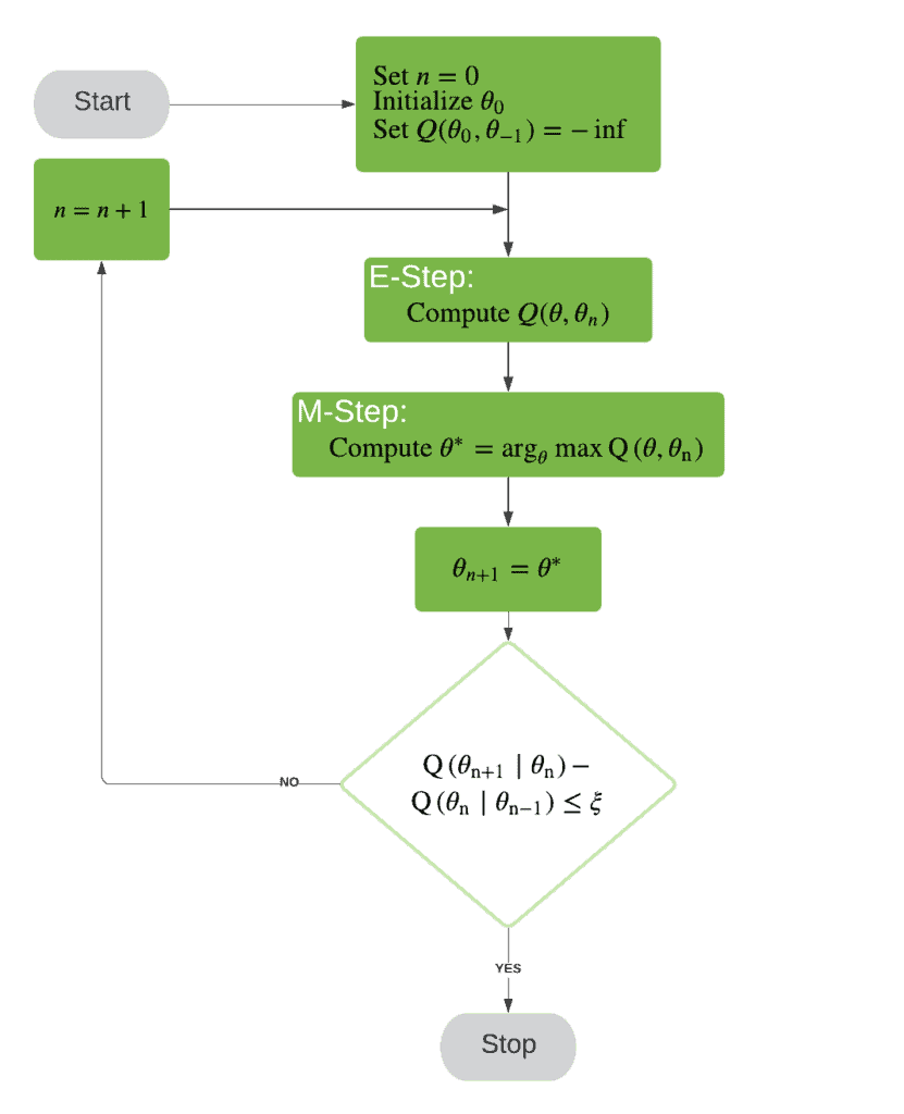
6. Flowchart
We can now summarize the whole procedure in a flowchart:
7. Conclusion
In this article, we reviewed some concepts like maximum likelihood estimation and then intuitively transitioned into an easy coin example of the expectation-maximization algorithm. We then tried to derive the algorithm and motivate why it is guaranteed to improve our estimation of the best parameters using Jensen’s inequality while putting everything together.