

Learn through the super-clean Baeldung Pro experience:
>> Membership and Baeldung Pro.
No ads, dark-mode and 6 months free of IntelliJ Idea Ultimate to start with.
Learn through the super-clean Baeldung Pro experience:
>> Membership and Baeldung Pro.
No ads, dark-mode and 6 months free of IntelliJ Idea Ultimate to start with.
Data structures are one of the major branches of computer science that defines the organization, management, and storage of data for efficient access and modification. There are numerous data structures available based on the storage, access, and usage types.
In this tutorial, we’ll look into several advanced data structures.
We call a data structure linear if its elements form a linear sequence. Let’s discuss several types of linear data structures.
A self-organizing list lets us reorder its elements based on certain algorithms to improve the average element access time. It is similar to a linked list except for the reorganizing capabilities.
In a linked list, the searching process requires comparing each element of the list with the item until the item is found or we reach the end of the list. Thus, in the worst-case scenario, we need to search  elements, where is the size of the list. A self-organizing list attempts to improve the average search time by moving the accessed elements towards the head of the list.
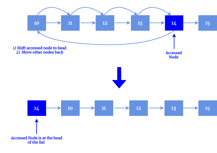
Let’s discuss several algorithms that decide the reorganizing process. We can start with the move to the front method.
In this technique, if an element is accessed, it is moved to the head of the list. This method has both merits and demerits. It is easy to implement as it simply moves an element if it is accessed. On the other hand, it can prioritize the infrequently accessed elements. For instance, if an uncommon element is accessed even once, it is moved to the head of the list, and given maximum priority even if it is not getting access again in the future. Thus, it can break the optimal structure of the list:
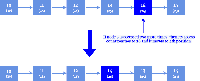
Next, we have a count method. In the count method, each method keeps track of the number of times it is searched. Nodes are ordered based on their count value in descending order:
A circular buffer or ring buffer is a data structure that uses a single fixed-size buffer as if were connected end-to-end. The name is because the buffer’s start and end are connected, and it looks like a circle.
One useful property of circular buffer over the non-circular data buffer (e.g., Stack) is that it does not need to have its elements shuffled around when one is consumed. If a non-circular buffer were used, then it would be necessary to shift all elements when one is consumed.
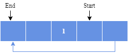
Initially, a circular buffer starts empty and has a defined length. In the following diagram, the buffer has a size of five:

Let’s assume that the value one is written in the center of a Circular Buffer. The exact starting location is not important in a Circular Buffer:
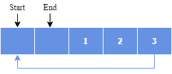
After that, imagine two more elements are added to the Circular Buffer — two & three — which is placed after one:
If two elements are removed, the two oldest values inside of the Circular Buffer would be removed. Circular Buffers use FIFO (First In, First Out) logic. In this example, one & two were the first to enter the Circular Buffer. They are the first to be removed, leaving three inside of the Buffer:
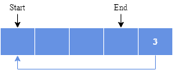
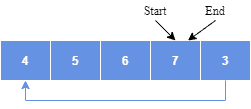
If the buffer has five elements, then it is full:
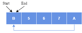
Another interesting property of the circular buffer is that when it is full and a subsequent write is performed, it starts overwriting the oldest data. In the current example, two more elements — A & B — are added, and they overwrite the three and four:
Circular buffering is an excellent choice for a queue that has a fixed maximum size. If a maximum size needs to be adopted for a queue, then a circular buffer is a completely ideal implementation as all queue operations are performed in constant time. However, expanding a circular buffer requires shifting memory, which is a costly operation. In such a scenario, a linked list approach could be a better approach.
A gap buffer is a data structure that lets us perform efficient insertion and deletion operations clustered near the same location. This is a popular data structure in the text editors where most of the text changes occur at or near the cursor’s current location. The text is stored in a large buffer in two contiguous segments, with a gap between them for inserting new text:
The quick brown fox [ ] over the lazy dogMoving the cursor involves copying text from one side of the gap to the other. An insert operation adds the new text at the end of the first segment, whereas a deletion deletes it.
Let us explain this with an example. The initial state is shown below:
The quick [ ] over the dogA user inserts a new text:
The quick brown fox jumps [ ] over the dogThe user moves the cursor after the word the:
The quick brown fox jumps over the [] dogThe user adds a new word named lazy, and the system creates a new gap:
The quick brown fox jumps over the lazy [] dogA text in a gap buffer is represented as two separate strings that take very little extra space. Thus, it can be searched and displayed very quickly, compared to more sophisticated data structures such as the linked lists. However, operations at different locations in the text and ones that fill the gap (i.e., requiring a new gap to be created) may require copying most of the text, which is especially inefficient for large files.
Gap buffers implementations assume that recopying text rarely occurs enough that its cost can be amortized over the more common cheap operations. This makes the gap buffer a simpler alternative to the Rope data structure for use in text editors.
A hashed array tree is a data structure that maintains an array of separate memory-fragments or leaves that store data elements. The major benefit of this data structure is that unlike dynamic arrays, which store elements in a contagious memory area, it reduces the amount of element copy otherwise needed due to automatic resizing.
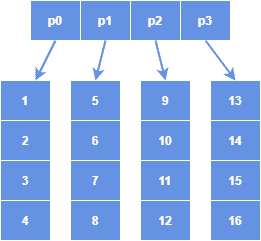
The top-level directory of a hashed array tree contains the power of two number of leaf arrays and are of the same size as the top-level directory. The reason for using the size as the power of two is for faster physical addressing through bit operations instead of using the arithmetic operations of quotient and remainder.
The structure of a hashed array tree resembles a hash table with a linked-list collision chain, which is the basis of its name. Besides, a full hashed array tree can hold a maximum of  number of elements, where m is the size of the top-level directory. In the above diagram, the top-level directory size is four. Thus, a maximum of 16 elements can be accommodated in the tree.
A non-linear data structure is the opposite of a linear data structure in which elements are not organized in a linear or continuous fashion. A tree or a heap is an example of a non-linear data structure. Let’s discuss a few other non-linear data structures in this section:
A rope is a tree data structure composed of smaller strings used to store and manipulate a long string. Rope, also knows as the cord is effective for this purpose. For instance, a text editing program can use a rope to represent a text so that it can manage the insert, delete, and update operations effectively:
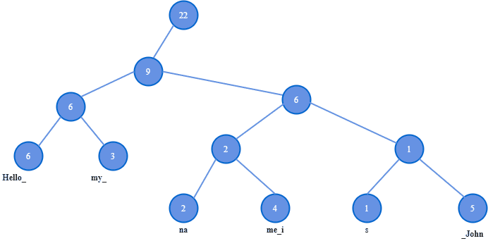
A rope is a type of binary tree in which each lead node holds a string and a length. Each node further up in the tree holds the sum of the length of all leaves in its left subtree. For example, the node with weight nine gets its value as its left subtree has the sum of length (Hello_) six and (my_) three.
A node with two children divides a string into two parts. The left subtree stores the first part of the string, the right subtree stores the second part of the string, and a node’s weight is the length of the first part.
A splay tree is a binary search tree with an additional property to quickly search the recently accessed elements again. Like the binary search tree, a splay tree performs the insert, look-up, and deletion in  time. For many sequences of non-random operations, the splay trees perform better than other search trees.
All normal operations of a Splay tree are based upon a basic operation, which is known as splaying. The splaying the tree for an element rearranges the tree so that the element in operation appears at the root of the tree. There are several ways this can be achieved. For instance, one can perform a basic binary search to find the element in operation in the tree and then use tree rotation techniques to move the element at the top of the tree. There are other top-down algorithms that can combine the search and the tree rotation in a single phase.
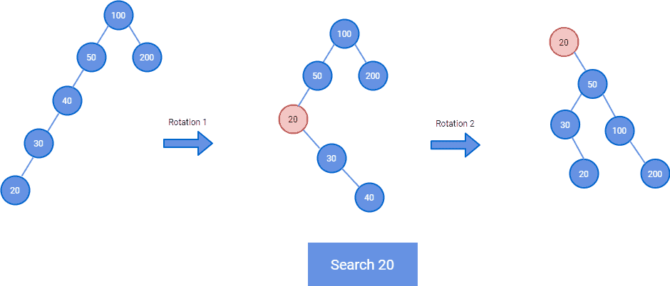
In the above diagram, we are searching the element 20 which is at the leaf node. At the end of the rotations, element 20 is moved to the root of the tree, and also the tree is balanced.
A binary heap is a heap data structure that takes the form of a binary tree and is commonly used to implement priority queues. A binary heap is a binary tree with two additional constraints:
A heap in which the parent key is greater than or equal to the child key is known as max-heaps. Whereas if the parent key is lesser than or equals to the child key, then it is known as min-heap.
In this article, we talked about several advanced data structures.
First, we explained a linear data structure and examined several candidates such as Self-organizing List, Circular Buffer, Gap Buffer, and Hashed array tree data structures.
Lastly, we learned about the non-linear data structure that includes trees, heaps, and graphs. In this category, we discussed Rope, Splay Tree, and Binary Heap data structures.