Guide to the Storage Engine in Apache Cassandra
Last updated: January 8, 2024


Mocking is an essential part of unit testing, and the Mockito library makes it easy to write clean and intuitive unit tests for your Java code.
Get started with mocking and improve your application tests using our Mockito guide:
Handling concurrency in an application can be a tricky process with many potential pitfalls. A solid grasp of the fundamentals will go a long way to help minimize these issues.
Get started with understanding multi-threaded applications with our Java Concurrency guide:
Spring 5 added support for reactive programming with the Spring WebFlux module, which has been improved upon ever since. Get started with the Reactor project basics and reactive programming in Spring Boot:
Since its introduction in Java 8, the Stream API has become a staple of Java development. The basic operations like iterating, filtering, mapping sequences of elements are deceptively simple to use.
But these can also be overused and fall into some common pitfalls.
To get a better understanding on how Streams work and how to combine them with other language features, check out our guide to Java Streams:
Explore Spring Boot 3 and Spring 6 in-depth through building a full REST API with the framework:
Yes, Spring Security can be complex, from the more advanced functionality within the Core to the deep OAuth support in the framework.
I built the security material as two full courses - Core and OAuth, to get practical with these more complex scenarios. We explore when and how to use each feature and code through it on the backing project.
You can explore the course here:
Spring Data JPA is a great way to handle the complexity of JPA with the powerful simplicity of Spring Boot.
Get started with Spring Data JPA through the guided reference course:
Refactor Java code safely — and automatically — with OpenRewrite.
Refactoring big codebases by hand is slow, risky, and easy to put off. That’s where OpenRewrite comes in. The open-source framework for large-scale, automated code transformations helps teams modernize safely and consistently.
Each month, the creators and maintainers of OpenRewrite at Moderne run live, hands-on training sessions — one for newcomers and one for experienced users. You’ll see how recipes work, how to apply them across projects, and how to modernize code with confidence.
Join the next session, bring your questions, and learn how to automate the kind of work that usually eats your sprint time.
Yes, we're now running our only Summer Sale. All Courses are 30% off until 20th July, 2026:
Yes, we're now running our only Summer Sale. All Courses are 30% off until 20th July, 2026:
1. Overview
Modern database systems are tailored to guarantee a set of capabilities such as reliability, consistency, high throughput, and so on by leveraging sophisticated storage engines for writing and reading data.
In this tutorial, we’ll dive deep into the internals of the storage engine used by Apache Cassandra, which is designed for write-heavy workloads while maintaining good performance for reads as well.
2. Log-Structured Merge-Tree (LSMT)
Apache Cassandra leverages a two-level Log-Structured Merge-Tree based data structure for storage. At a high level, there are two tree-like components in such an LSM tree, an in-memory cache component (C0) and an on-disk component (C1):
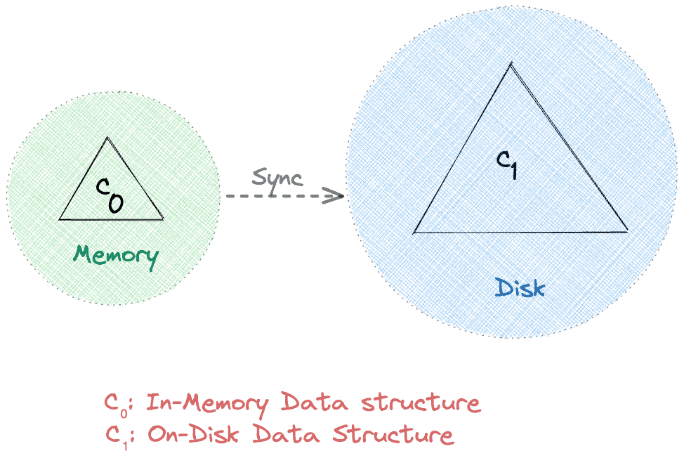
Reading and writing directly from memory is usually faster than the disk. Therefore, by design, all requests hit C0 before reaching out to C1. Moreover, a sync operation persists data from C0 to C1 periodically. As a result, it uses network bandwidth efficiently by reducing the I/O operations.
In the following sections, we’ll learn more about the C0 and C1 data structures of the two-level LSM tree in Apache Cassandra, commonly known as MemTable and SSTable, respectively.
3. MemTable
As the name suggests, MemTable is a memory-resident data structure such as a Red-black tree with self-balancing binary search tree properties. As a result, all the read and write operations, namely, search, insert, update, and delete, are achievable with O(log n) time complexity.
Being an in-memory mutable data structure, MemTable makes all the writes sequential and allows for fast write operations. Further, due to the typical constraints of physical memory, such as limited capacity and volatile nature, we need to persist data from MemTable to disk:
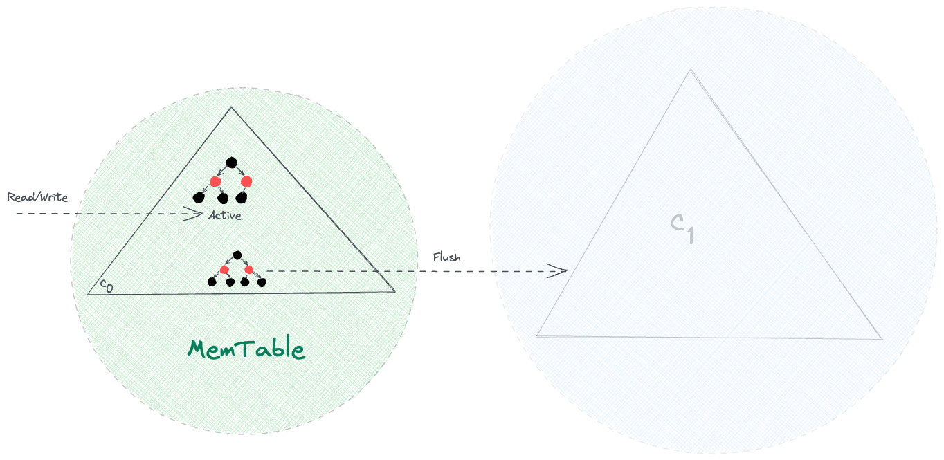
Once the size of MemTable reaches a threshold value, all the r/w requests switch to a new MemTable, while the old one is discarded after flushing it onto the disk.
So far, so good! We can handle a large number of writes efficiently. However, what happens, if the node crashes before a flush operation? Well, it’s simple — we’d lose the data that isn’t flushed to disk yet.
In the next section, we’ll see how Apache Cassandra solves this problem by using the concept of Write-Ahead Logs (WAL).
4. Commit Log
Apache Cassandra defers the flush operation that persists data from memory to disk. Hence, an unexpected node or process crash can lead to data loss.
Durability is a must-have capability for any modern database system, and Apache Cassandra is no exception. It guarantees durability by ensuring all writes persist onto the disk in an append-only file called Commit Log. Thereafter, it uses MemTable as a write-back cache in the write-path:

We must note that append-only operations are fast as they avoid random seeks on the disk. So, the Commit Log brings durability capability without compromising the performance of writes. Further, Apache Cassandra refers to the Commit Log only during a crash recovery scenario, while the regular read requests don’t go to the Commit Log.
5. SSTable
Sorted String Table (SSTable) is the disk-resident component of the LSM tree used by the Apache Cassandra storage engine. It derives its name from a similar data structure, first used by Google’s BigTable database, and indicates that the data is available in a sorted format. Generally speaking, each flush operation from the MemTable generates a new immutable segment in the SSTable.
Let’s try to visualize how an SSTable would look while containing data about the count of various animals kept in a zoo:

Though the segments are sorted by keys, nevertheless, the same key could be present in multiple segments. So if we’ve to look for a specific key, we need to start our search from the latest segment and return the result as soon as we find it.
With such a strategy, read operations for the recently written keys would be fast. However, in the worst case, the algorithm executes with an O(N*log(K)) time complexity, where N is the total number of segments, and K is the segment size. As K is a constant, we can say that the overall time complexity is O(N), which is not efficient.
In the following few sections, we’ll learn how Apache Cassandra optimizes the read operations for SSTable.
6. Sparse Index
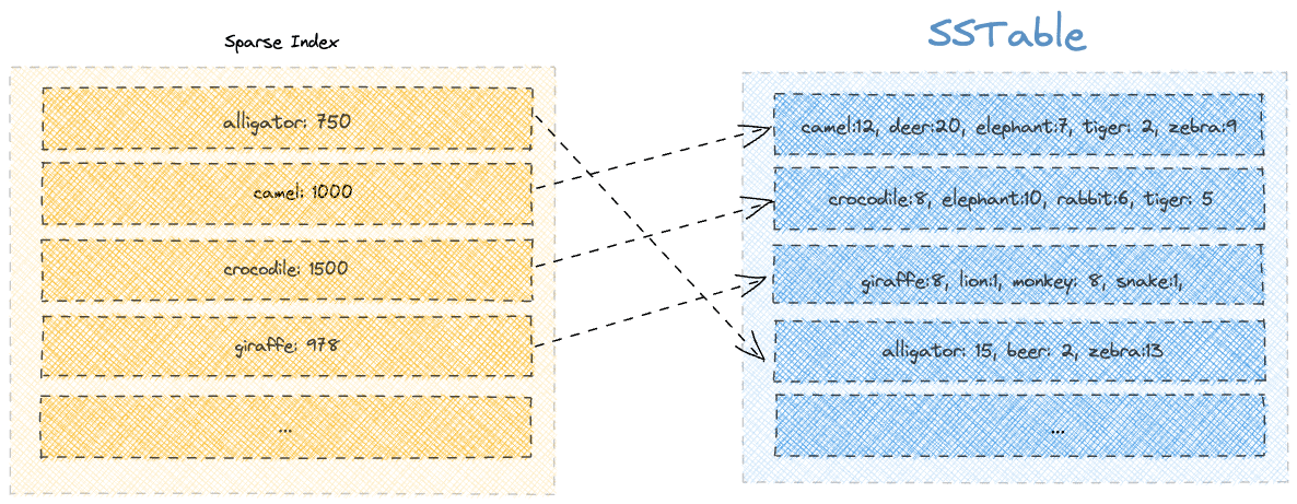
Apache Cassandra maintains a sparse index to limit the number of segments it needs to scan while looking for a key.
Each entry in the sparse index contains the first member of a segment, along with its page offset position on the disk. Further, the index is maintained in memory as a B-Tree data structure so that we can search for an offset in the index with O(log(K)) time complexity.
Let’s say we want to search for the key “beer.” We’ll start by searching for all the keys in the sparse index that’d come before the word “beer.” After that, using the offset value, we’ll look into only a limited number of segments. In this case, we’ll look into the fourth segment where the first key is “alligator”:
On the other hand, if we had to search for an absent key such as “kangaroo,” we’d have to look through all the segments in vain. So, we realize that using a sparse index optimizes the search to a limited extent.
Moreover, we should note that SSTable allows the same key to be present in different segments. Therefore, with time, more and more updates will happen for the same key, thereby creating duplicate keys in sparse index too.
In the following sections, we’ll learn how Apache Cassandra addresses these two problems with the help of bloom filters and compaction.
7. Bloom Filter
Apache Cassandra optimizes the read queries using a probabilistic data structure known as a bloom filter. Simply put, it optimizes the search by first performing a membership check for a key using a bloom filter.
So, by attaching a bloom filter to each segment of the SSTable, we’d get significant optimizations for our read queries, especially for keys that aren’t present in a segment:

As bloom filters are probabilistic data structures, we could get “Maybe” as a response, even for missing keys. However, if we get “No” as a response, we can be sure that the key’s definitely missing.
Despite their limitations, we can plan to improve the accuracy of bloom filters by allocating larger storage space for them.
8. Compaction
Despite using bloom filters and a sparse index, the performance of the read queries would degrade with time. That’s because the number of segments containing different versions of a key will likely grow with each MemTable flush operation.
To solve the issue, Apache Cassandra runs a background process of compaction that merges smaller sorted segments into larger segments while keeping only the latest value for each key. So, the compaction process gives the dual benefit of faster reads with lesser storage.
Let’s see what a single run of compaction would look like on our existing SSTable:
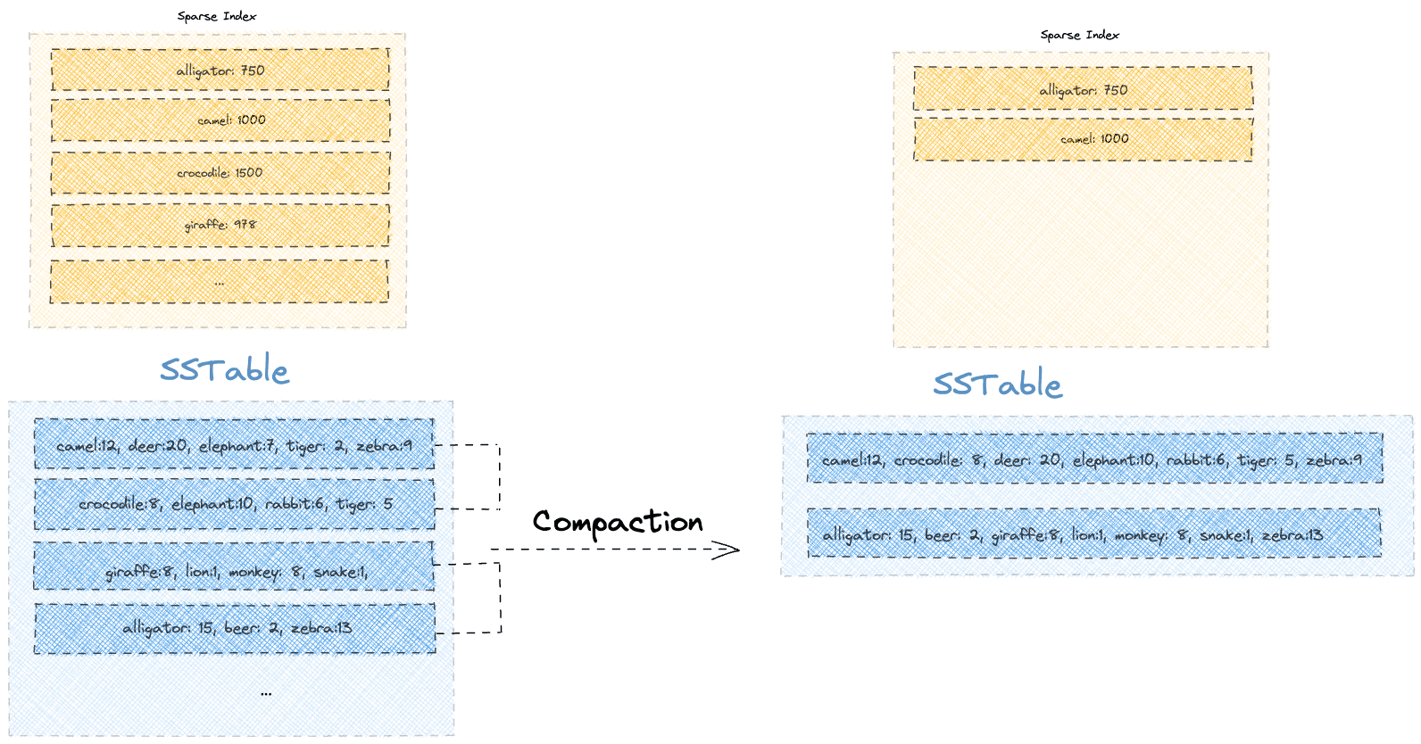
We notice that the compaction operation reclaimed some space by keeping only the latest version. For instance, old versions of keys such as “elephant” and “tiger” are no longer present, thereby freeing up disk space.
Additionally, the compaction process enables the hard deletion of keys. While a delete operation would mark a key with a tombstone, the actual deletion is deferred until compaction.
9. Conclusion
In this article, we explored the internal components of Apache Cassandra’s storage engine. While doing so, we learned about advanced data structure concepts such as LSM Tree, MemTable, and SSTable. Moreover, we also learned a few optimization techniques using Write-Ahead Logging, Bloom Filters, Sparse Index, and Compaction.