B-tree Data Structure | Baeldung on Computer Science

1. Overview

In this tutorial, we’ll discuss a self-balancing tree data structure: B-tree. We’ll present the properties and various operations of the B-tree.

2. Introduction

B-tree is a tree data structure. In this tree structure, data is stored in the form of nodes and leaves. B-tree is known as a self-balanced sorted search tree. It’s a more complex and updated version of the binary search tree (BST) with additional tree properties.

The main difference between a binary search tree and a B-tree is that a B-tree can have multiple children nodes for a parent node. However, a binary search tree can contain only two child nodes for a parent node.

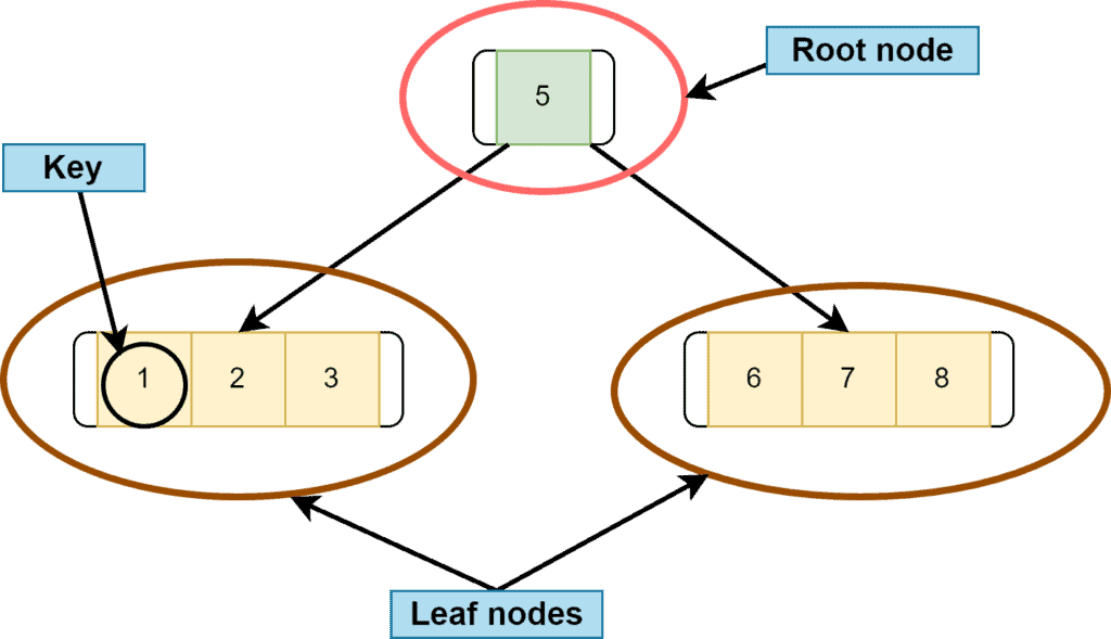
Unlike a binary search tree, a B-tree can have multiple keys in a node. The number of keys and the number of children for any node depends on the order of the B-tree. Keys are the values that are stored at any node. Let’s take a look at an example of B-tree:

3. Properties

Some properties of the B-tree are similar to BST. The parent node’s key is always greater than the key values of the left subtree nodes. Similarly, the parent node’s key is always less than the key values of the right subtree nodes.

It can have multiple keys for a single node. A single node can have more than two children.

All the leaf nodes must be at the same level. A leaf node is a node that doesn’t have any child nodes.

Suppose the order of a B-tree is $N$ . It means every node can have a maximum of $N$ children. Therefore, every node can have maximum $\textbf{(N-1)}$ keys and minimum $\textbf{\{(N/2)-1\}}$ keys except the root node.

Let’s take a B-tree of order $N = 6$ . According to the properties of the B-tree, any node can have a maximum of $(N-1)$ keys. Hence $5$ keys in this case. Furthermore, any node can have minimum $\{(N/2)-1\}$ keys. Hence, $\{(6/2) -1\} = 2$ keys.

4. B-tree Operations

Like any other tree data structure, three primary operations can be performed on a B-tree: searching, insertion, and deletion. Let’s discuss each operation one by one.

4.1. Searching

The structure of the B-tree is similar to the binary search tree, with some added properties. Hence, the searching operation in a B-tree works the same as a BST. Initially, we start searching from a root node.

We either go to the left or right subtree from the root node, depending on the key value of the node we want to search. On top of this, in a B-tree, we have several decisions, as there can be more than two branches for a node.

The searching time complexity of a B-tree in the best, as well as the worst-case, is $\textbf{\mathcal{O}(logn)}$ , where $n$ denotes the total number of elements in a B-tree.

4.2. Insertion

Insertion is the operation in which we insert or add elements in a B-tree. During this process, we need to keep some points in mind. We can’t insert any element at the root node of a B-tree. We have to start inserting elements from the leaf node.

Additionally, while inserting a node in a B-tree, we must check the maximum number of keys at any node and add elements in ascending order.

Let’s take the example of inserting some nodes in an empty B-tree. Here, we want to insert $10$ nodes in a empty B-tree: $(1, 2, 3, 4, 5, 6, 7, 8, 9, 10)$ . Let’s assume the order of the B-tree is $\mathsf{3}$ . Hence, the maximum number of children a node can contain is $\mathsf{3}$ . Additionally, the maximum and the minimum number of keys for a node, in this case, would be $\mathsf{2}$ and $\mathsf{1}$ (rounded off).

While inserting any element, we must remember that we can only insert values in ascending order. Moreover, we always insert elements at the leaf node so that the B-tree always grows in the upward direction.

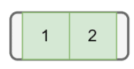
Let’s start the insertion process with nodes $\textbf{1}$ and $\textbf{2}$ :

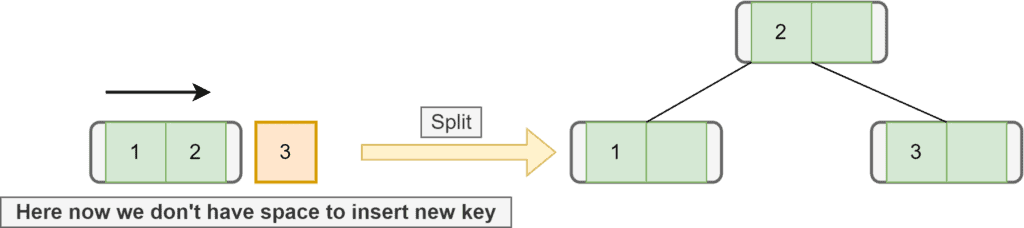
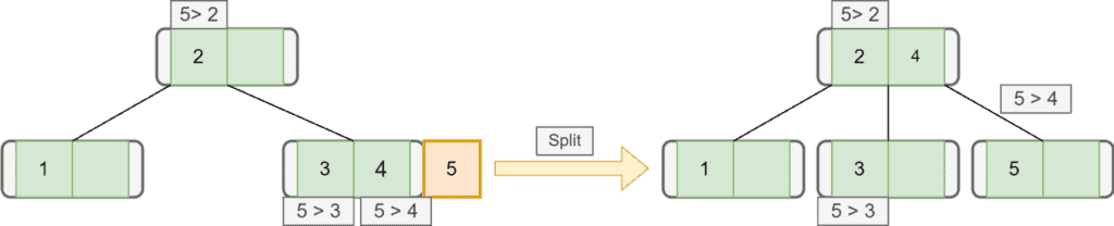
Next, we want to insert node $\textbf{3}$ . But there’s no space for inserting new elements in that leaf node as the maximum key a node can contain is $2$ here. Therefore, we need to split the node. To split the node, we take the median key and move that key upward:

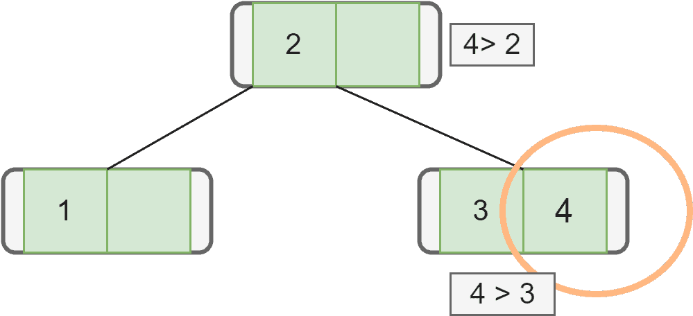
Now we want to insert the next element $\textbf{4}$ . As $\mathsf{4}$ is greater than $\mathsf{2}$ , we first go to the right subtree. In the right subtree, there’s a node with key $\mathsf{3}$ . The key of the incoming node is greater than $\mathsf{3}$ . Hence, we’ll add this node to the right of $\mathsf{3}$ :

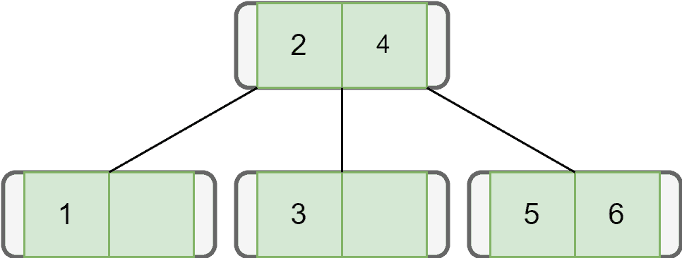
Let’s insert the next node with key $\textbf{5}$ . We first check the root, and as $\mathsf{5}$ is greater than $\mathsf{2}$ , we go to the right subtree. In the right subtree, we see $\mathsf{5}$ is greater than $\mathsf{3}$ and $\mathsf{4}$ . Hence, we insert $\mathsf{5}$ on the right side of $\mathsf{4}$ . But again, there’s not enough space. Therefore, we split it and move the median of $\mathsf{3, 4, 5}$ that is $\mathsf{4}$ , to the upper node:

Similarly, we insert our next node with key $\textbf{6}$ :

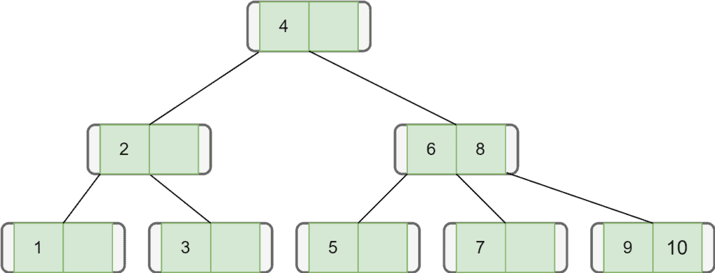
Finally, let’s add all the remaining nodes one by one, following the properties of the B-tree:

The time complexity of the insertion process of a B-tree is $\textbf{\mathcal{O}(logn)}$ .

4.3. Deletion

Deletion is the process in which we remove keys from a B-tree. During this process, we need to maintain B-tree properties. After deleting any key, the tree must be arranged again to follow B-tree properties. Additionally, we need to search that key in the B-tree before deletion.

There can be two possible situations while deleting a key from a B-tree. Firstly, the key we want to delete is in a leaf node. Secondly, the key we want to delete is in the internal node.

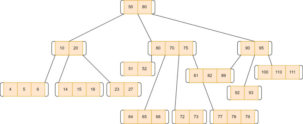
Let’s take an example of deletion from the B-tree: Here, we’re taking a B-tree of order $\mathsf{5}$ . The maximum number of children a node can contain is $\mathsf{5}$ . Additionally, the maximum and the minimum number of keys for a node, in this case, would be $\mathsf{4}$ and $\mathsf{2}$ :

If the target key’s leaf node contains more than the minimum required keys, we don’t have to worry about anything. We need to delete the target key. After deletion, it’ll still be a complete B-tree.

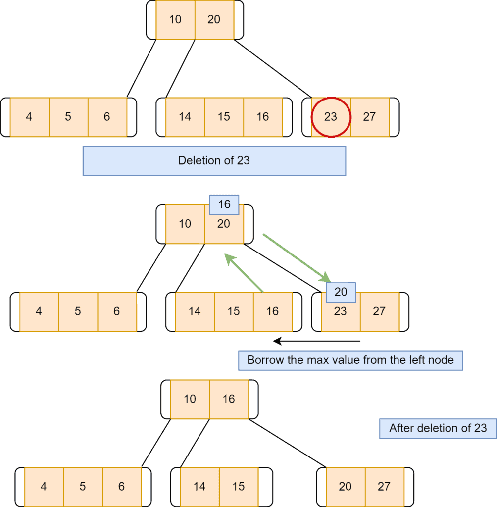
If the target key’s leaf node contains only the minimum number of keys, we can’t simply delete the key. Because if we do so, it’ll violate the condition of the B-tree. In such a case, borrow the key from the immediate left node if that node has more than the minimum required keys.

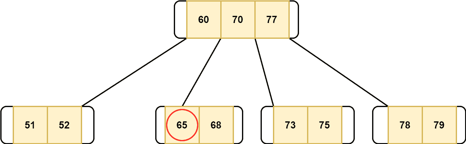
We’ll transfer the maximum value of the left node to its parent node. After that, the key with greater value will be transferred to the borrower node. Moreover, we can remove the target key from the node. Let’s say we want to remove a node with key $\mathsf{23}$ :

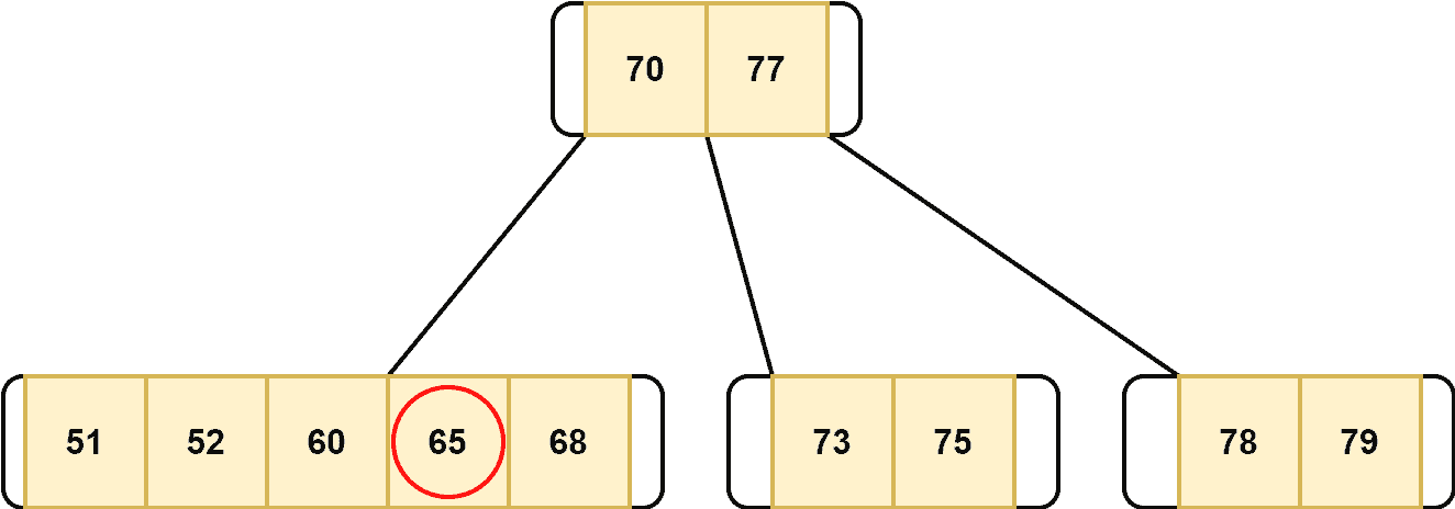
Another possible way is to borrow the key from the immediate right node if that node has more than the minimum required keys. We’ll transfer the minimum value of the right node to its parent node. The smaller key value will be transferred to the borrower node. After that, we can remove the target key from the node. Let’s say we want to remove a node with key $\mathsf{72}$ :

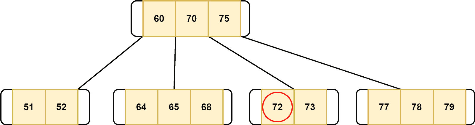
Thus, if we remove the key $\mathsf{72}$ from node 3, it’ll left with one key. However, the minimum number of keys one node should contain is $3$ . Hence, as soon as we delete the key $72$ , we need to add one key to node 3:

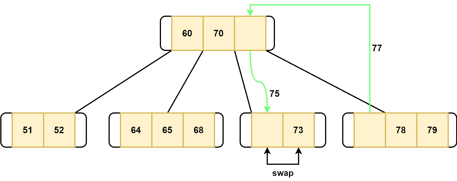
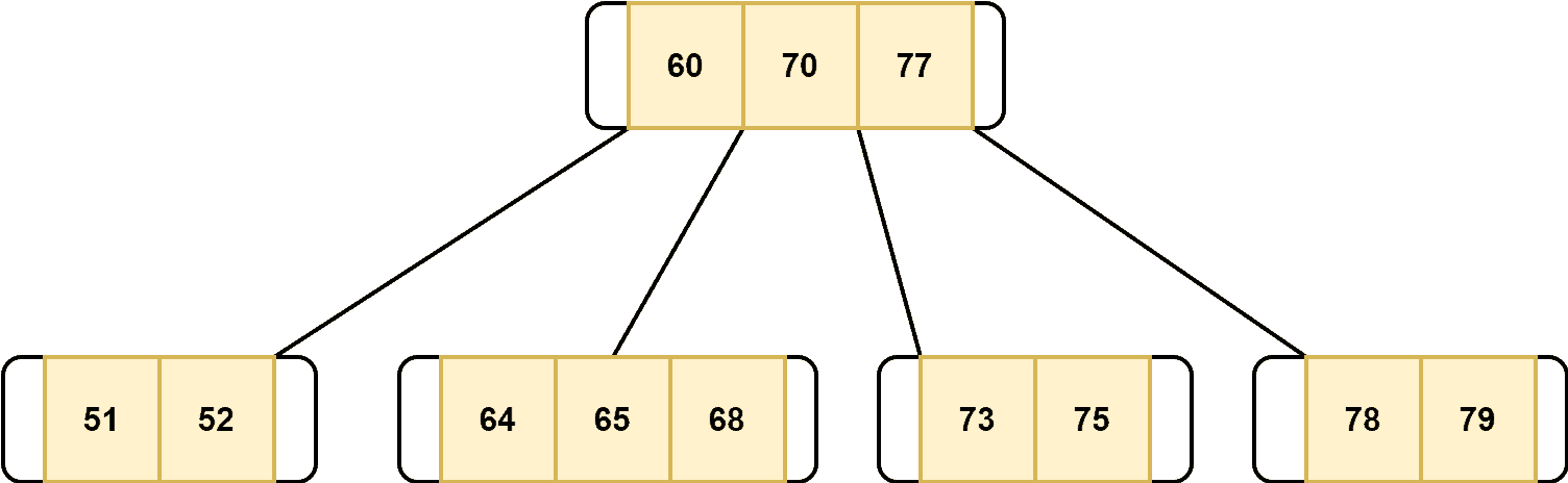
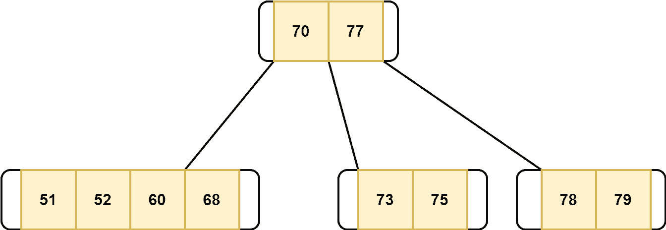
depicting all the operations when deleting the key 72

Here, we perform three operations. First, we replace the highest key of the parent with the lowest key from node 4. Furthermore, we filled node 3 with the highest key of the parent node. Finally, the keys of node 3 are swapped. Let’s take a look at the B-tree structure after we delete the key $72$ :

Final structure of B-tree after deletion of 72

Now, let’s discuss the scenario when neither the left sibling nor the right sibling of the target key’s node has more than the minimum required keys. In such a case, we need to merge two nodes. Out of two nodes, one node should contain our target node’s key. While merging, we also need to consider the parent nodes as well.

Suppose we want to delete a node with a key of $\textbf{65}$ :

As we can see, its sibling nodes don’t contain more than the minimum number of keys. Hence, to delete the key $65$ , the first step is to merge the nodes 1 and 2. Additionally, when merging the nodes, we need to remove the key $60$ from the parent node and add it to the merged node:

After merging the nodes, we delete our target node:

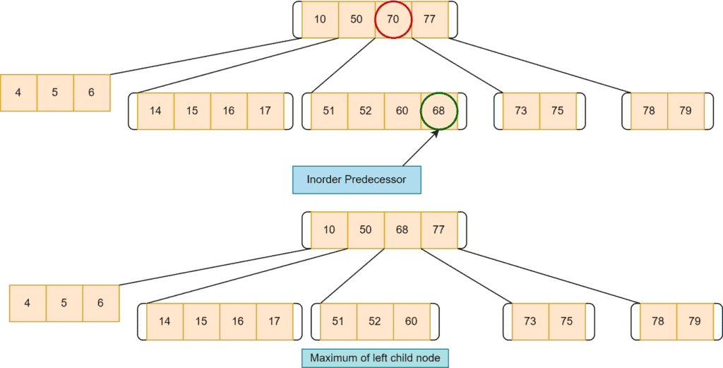
Now, let’s discuss the case when the target key is at an internal node:

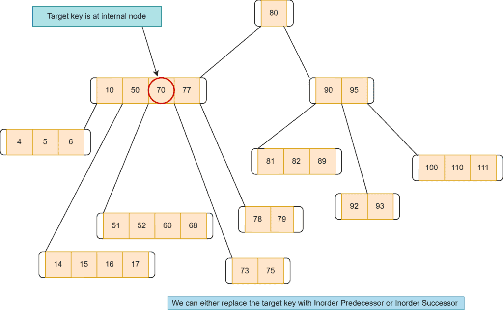
In such a case, the first possible option is to replace the target key with its in-order predecessor. Here, we take the left node of the target key, select the highest value key, and replace that with the target key. Here we want to delete node $\mathsf{70}$ :

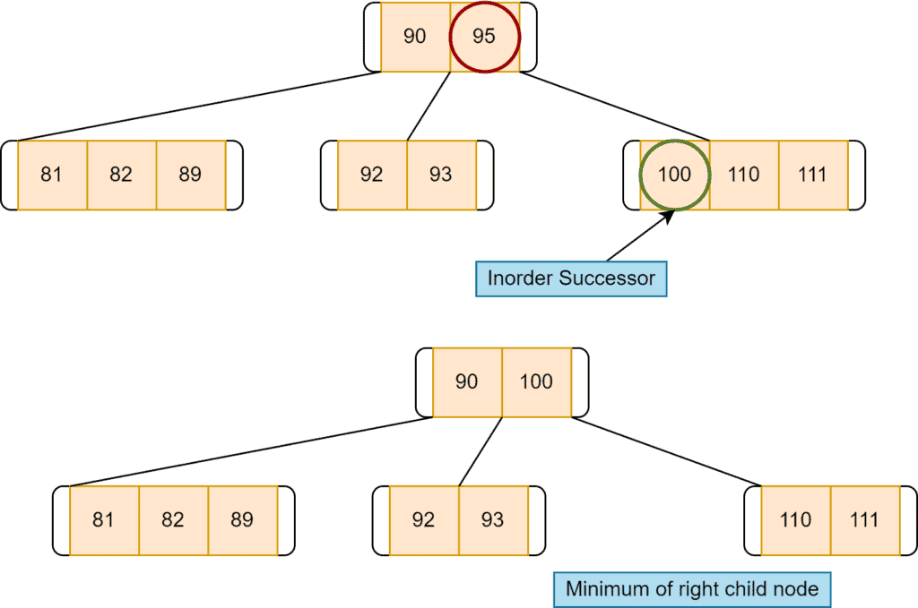
If the left doesn’t have more than the minimum required keys, we replace the target key with its in-order successor. Here, we’ll take the right node of the target key, select the lowest value key and replace that with the target key:

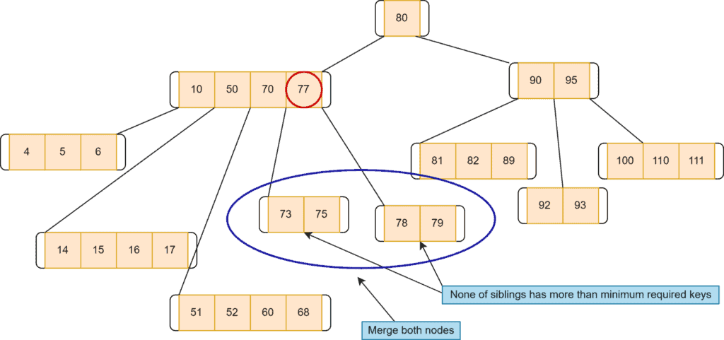
If the target key’s inorder successor node and inorder predecessor node don’t have more than the minimum number of the required key, we need to merge two adjacent nodes. For example, deletion of $\mathsf{77}$ :

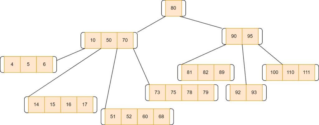
After the deletion of 77:

The time complexity of the deletion process of a B-tree is $\textbf{\mathcal{O}(logn)}$ .

6. Conclusion

B-Tree is a widely used data structure for storing a large amount of data. In this tutorial, we discussed the B-tree in detail. We presented the properties and operations with examples.

Full Archive

About Baeldung

Core Concepts

Operating Systems

Artificial Intelligence

Graph Theory

Latex