

1. Introduction
In this tutorial, we’ll learn how to use Atlas Search functionalities using the Java MongoDB driver API. By the end, we’ll have a grasp on creating queries, paginating results, and retrieving meta-information. Also, we’ll cover refining results with filters, adjusting result scores, and selecting specific fields to be displayed.
2. Scenario and Setup
MongoDB Atlas has a free forever cluster that we can use to test all features. To showcase Atlas Search functionalities, we’ll only need a service class. We’ll connect to our collection using MongoTemplate.
2.1. Dependencies
First, to connect to MongoDB, we’ll need spring-boot-starter-data-mongodb:
<dependency>
    <groupId>org.springframework.boot</groupId>
    <artifactId>spring-boot-starter-data-mongodb</artifactId>
    <version>3.1.2</version>
</dependency>
2.2. Sample Dataset
Throughout this tutorial, we’ll use the movies collection from MongoDB Atlas’s sample_mflix sample dataset to simplify examples. It contains data about movies since the 1900s, which will help us showcase the filtering capabilities of Atlas Search.
2.3. Creating an Index With Dynamic Mapping
For Atlas Search to work, we need indexes. These can be static or dynamic. A static index is helpful for fine-tuning, while a dynamic one is an excellent general-purpose solution. So, let’s start with a dynamic index.
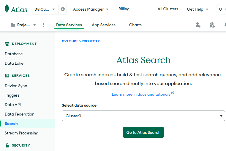
There are a few ways to create search indexes (including programmatically); we’ll use the Atlas UI. There, we can do this by accessing Search from the menu, selecting our cluster, then clicking Go to Atlas Search:
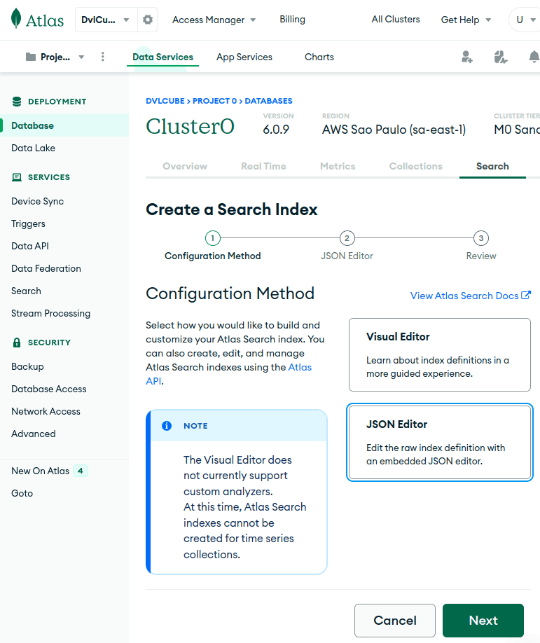
After clicking on Create Search Index, we’ll choose the JSON Editor to create our index, then click Next:
Finally, on the next screen, we choose our target collection, a name for our index, and input our index definition:
{
    "mappings": {
        "dynamic": true
    }
}
We’ll use the name idx-queries for this index throughout this tutorial. Note that if we name our index default, we don’t need to specify its name when creating queries. Most importantly, dynamic mappings are a simple choice for more flexible, frequently changing schemas.
By setting mappings.dynamic to true, Atlas Search automatically indexes all dynamically indexable and supported field types in a document. While dynamic mappings provide convenience, especially when the schema is unknown, they tend to consume more disk space and might be less efficient compared to static ones.
2.4. Our Movie Search Service
We’ll base our examples on a service class containing some search queries for our movies, extracting interesting information from them. We’ll slowly build them up to more complex queries:
@Service
public class MovieAtlasSearchService {

    private final MongoCollection<Document> collection;

    public MovieAtlasSearchService(MongoTemplate mongoTemplate) {
        MongoDatabase database = mongoTemplate.getDb();
        this.collection = database.getCollection("movies");
    }

    // ...
}
All we need is a reference to our collection for future methods.
3. Constructing a Query
Atlas Search queries are created via pipeline stages, represented by a List<Bson>. The most essential stage is Aggregates.search(), which receives a SearchOperator and, optionally, a SearchOptions object. Since we called our index idx-queries instead of default, we must include its name with SearchOptions.searchOptions().index(). Otherwise, we’ll get no errors and no results.
Many search operators are available to define how we want to conduct our query. In this example, we’ll find movies by tags using SearchOperator.text(), which performs a full-text search. We’ll use it to search the contents of the fullplot field with SearchPath.fieldPath(). We’ll omit static imports for readability:
public Collection<Document> moviesByKeywords(String keywords) {
    List<Bson> pipeline = Arrays.asList(
        search(
          text(
            fieldPath("fullplot"), keywords
          ),
          searchOptions()
            .index("idx-queries")
        ),
        project(fields(
          excludeId(),
          include("title", "year", "fullplot", "imdb.rating")
        ))
    );

    return collection.aggregate(pipeline)
      .into(new ArrayList<>());
}
Also, the second stage in our pipeline is Aggregates.project(), which represents a projection. If not specified, our query results will include all the fields in our documents. But we can set it and choose which fields we want (or don’t want) to appear in our results. Note that specifying a field for inclusion implicitly excludes all other fields except the _id field. So, in this case, we’re excluding the _id field and passing a list of the fields we want. Note we can also specify nested fields, like imdb.rating.
To execute the pipeline, we call aggregate() on our collection. This returns an object we can use to iterate on results. Finally, for simplicity, we call into() to iterate over results and add them to a collection, which we return. Note that a big enough collection can exhaust the memory in our JVM. We’ll see how to eliminate this concern by paginating our results later on.
Most importantly, pipeline stage order matters. We’ll get an error if we put the project() stage before search().
Let’s take a look at the first two results of calling moviesByKeywords(“space cowboy”) on our service:
[
    {
        "title": "Battle Beyond the Stars",
        "fullplot": "Shad, a young farmer, assembles a band of diverse mercenaries in outer space to defend his peaceful planet from the evil tyrant Sador and his armada of aggressors. Among the mercenaries are Space Cowboy, a spacegoing truck driver from Earth; Gelt, a wealthy but experienced assassin looking for a place to hide; and Saint-Exmin, a Valkyrie warrior looking to prove herself in battle.",
        "year": 1980,
        "imdb": {
            "rating": 5.4
        }
    },
    {
        "title": "The Nickel Ride",
        "fullplot": "Small-time criminal Cooper manages several warehouses in Los Angeles that the mob use to stash their stolen goods. Known as \"the key man\" for the key chain he always keeps on his person that can unlock all the warehouses. Cooper is assigned by the local syndicate to negotiate a deal for a new warehouse because the mob has run out of storage space. However, Cooper's superior Carl gets nervous and decides to have cocky cowboy button man Turner keep an eye on Cooper.",
        "year": 1974,
        "imdb": {
            "rating": 6.7
        }
    },
    (...)
]
3.1. Combining Search Operators
It’s possible to combine search operators using SearchOperator.compound(). In this example, we’ll use it to include must and should clauses. A must clause contains one or more conditions for matching documents. On the other hand, a should clause contains one or more conditions that we’d prefer our results to include.
This alters the score so the documents that meet these conditions appear first:
public Collection<Document> late90sMovies(String keywords) {
    List<Bson> pipeline = asList(
        search(
          compound()
            .must(asList(
              numberRange(
                fieldPath("year"))
                .gteLt(1995, 2000)
            ))
            .should(asList(
              text(
                fieldPath("fullplot"), keywords
              )
            )),
          searchOptions()
            .index("idx-queries")
        ),
        project(fields(
          excludeId(),
          include("title", "year", "fullplot", "imdb.rating")
        ))
    );

    return collection.aggregate(pipeline)
      .into(new ArrayList<>());
}
We kept the same searchOptions() and projected fields from our first query. But, this time, we moved text() to a should clause because we want the keywords to represent a preference, not a requirement.
Then, we created a must clause, including SearchOperator.numberRange(), to only show movies from 1995 to 2000 (exclusive) by restricting the values on the year field. This way, we only return movies from that era.
Let’s see the first two results for hacker assassin:
[
    {
        "title": "Assassins",
        "fullplot": "Robert Rath is a seasoned hitman who just wants out of the business with no back talk. But, as things go, it ain't so easy. A younger, peppier assassin named Bain is having a field day trying to kill said older assassin. Rath teams up with a computer hacker named Electra to defeat the obsessed Bain.",
        "year": 1995,
        "imdb": {
            "rating": 6.3
        }
    },
    {
        "fullplot": "Thomas A. Anderson is a man living two lives. By day he is an average computer programmer and by night a hacker known as Neo. Neo has always questioned his reality, but the truth is far beyond his imagination. Neo finds himself targeted by the police when he is contacted by Morpheus, a legendary computer hacker branded a terrorist by the government. Morpheus awakens Neo to the real world, a ravaged wasteland where most of humanity have been captured by a race of machines that live off of the humans' body heat and electrochemical energy and who imprison their minds within an artificial reality known as the Matrix. As a rebel against the machines, Neo must return to the Matrix and confront the agents: super-powerful computer programs devoted to snuffing out Neo and the entire human rebellion.",
        "imdb": {
            "rating": 8.7
        },
        "year": 1999,
        "title": "The Matrix"
    },
    (...)
]
4. Scoring the Result Set
When we query documents with search(), the results appear in order of relevance. This relevance is based on the calculated score, from highest to lowest. This time, we’ll modify late90sMovies() to receive a SearchScore modifier to boost the relevance of the plot keywords in our should clause:
public Collection<Document> late90sMovies(String keywords, SearchScore modifier) {
    List<Bson> pipeline = asList(
        search(
          compound()
            .must(asList(
              numberRange(
                fieldPath("year"))
                .gteLt(1995, 2000)
            ))
            .should(asList(
              text(
                fieldPath("fullplot"), keywords
              )
              .score(modifier)
            )),
          searchOptions()
            .index("idx-queries")
        ),
        project(fields(
          excludeId(),
          include("title", "year", "fullplot", "imdb.rating"),
          metaSearchScore("score")
        ))
    );

    return collection.aggregate(pipeline)
      .into(new ArrayList<>());
}
Also, we include metaSearchScore(“score”) in our fields list to see the score for each document in our results. For example, we can now multiply the relevance of our “should” clause by the value of the imdb.votes field like this:
late90sMovies(
  "hacker assassin",
  SearchScore.boost(fieldPath("imdb.votes"))
)
And this time, we can see that The Matrix comes first, thanks to the boost:
[
    {
        "fullplot": "Thomas A. Anderson is a man living two lives (...)",
        "imdb": {
            "rating": 8.7
        },
        "year": 1999,
        "title": "The Matrix",
        "score": 3967210.0
    },
    {
        "fullplot": "(...) Bond also squares off against Xenia Onatopp, an assassin who uses pleasure as her ultimate weapon.",
        "imdb": {
            "rating": 7.2
        },
        "year": 1995,
        "title": "GoldenEye",
        "score": 462604.46875
    },
    (...)
]
4.1. Using a Score Function
We can achieve greater control by using a function to alter the score of our results. Let’s pass a function to our method that adds the value of the year field to the natural score. This way, newer movies end up with a higher score:
late90sMovies(keywords, function(
  addExpression(asList(
    pathExpression(
      fieldPath("year"))
      .undefined(1),
    relevanceExpression()
  ))
));
That code starts with a SearchScore.function(), which is a SearchScoreExpression.addExpression() since we want an add operation. Then, since we want to add a value from a field, we use a SearchScoreExpression.pathExpression() and specify the field we want: year. Also, we call undefined() to determine a fallback value for year in case it’s missing. In the end, we call relevanceExpression() to return the document’s relevance score, which is added to the value of year.
When we execute that, we’ll see “The Matrix” now appears first, along with its new score:
[
    {
        "fullplot": "Thomas A. Anderson is a man living two lives (...)",
        "imdb": {
            "rating": 8.7
        },
        "year": 1999,
        "title": "The Matrix",
        "score": 2003.67138671875
    },
    {
        "title": "Assassins",
        "fullplot": "Robert Rath is a seasoned hitman (...)",
        "year": 1995,
        "imdb": {
            "rating": 6.3
        },
        "score": 2003.476806640625
    },
    (...)
]
That’s useful for defining what should have greater weight when scoring our results.
5. Getting Total Rows Count From Metadata
If we need to get the total number of results in a query, we can use Aggregates.searchMeta() instead of search() to retrieve metadata information only. With this method, no documents are returned. So, we’ll use it to count the number of movies from the late 90s that also contain our keywords.
For meaningful filtering, we’ll also include the keywords in our must clause:
public Document countLate90sMovies(String keywords) {
    List<Bson> pipeline = asList(
        searchMeta(
          compound()
            .must(asList(
              numberRange(
                fieldPath("year"))
                .gteLt(1995, 2000),
              text(
                fieldPath("fullplot"), keywords
              )
            )),
          searchOptions()
            .index("idx-queries")
            .count(total())
        )
    );

    return collection.aggregate(pipeline)
      .first();
}
This time, searchOptions() includes a call to SearchOptions.count(SearchCount.total()), which ensures we get an exact total count (instead of a lower bound, which is faster depending on the collection size). Also, since we expect a single object in the results, we call first() on aggregate().
Finally, let’s see what is returned for countLate90sMovies(“hacker assassin”):
{
    "count": {
        "total": 14
    }
}
This is useful for getting information about our collection without including documents in our results.
6. Faceting on Results
In MongoDB Atlas Search, a facet query is a feature that allows retrieving aggregated and categorized information about our search results. It helps us analyze and summarize data based on different criteria, providing insights into the distribution of search results.
Also, it enables grouping search results into different categories or buckets and retrieving counts or additional information about each category. This helps answer questions like “How many documents match a specific category?” or “What are the most common values for a certain field within the results?”
6.1. Creating a Static Index
In our first example, we’ll create a facet query to give us information about genres from movies since the 1900s and how these relate. We’ll need an index with facet types, which we can’t have when using dynamic indexes.
So, let’s start by creating a new search index in our collection, which we’ll call idx-facets. Note that we’ll keep dynamic as true so we can still query the fields that are not explicitly defined:
{
  "mappings": {
    "dynamic": true,
    "fields": {
      "genres": [
        {
          "type": "stringFacet"
        },
        {
          "type": "string"
        }
      ],
      "year": [
        {
          "type": "numberFacet"
        },
        {
          "type": "number"
        }
      ]
    }
  }
}
We started by specifying that our mappings aren’t dynamic. Then, we selected the fields we were interested in for indexing faceted information. Since we also want to use filters in our query, for each field, we specify an index of a standard type (like string) and one of a faceted type (like stringFacet).
6.2. Running a Facet Query
Creating a facet query involves using searchMeta() and starting a SearchCollector.facet() method to include our facets and an operator for filtering results. When defining the facets, we have to choose a name and use a SearchFacet method that corresponds to the type of index we created. In our case, we define a stringFacet() and a numberFacet():
public Document genresThroughTheDecades(String genre) {
    List pipeline = asList(
      searchMeta(
        facet(
          text(
            fieldPath("genres"), genre
          ),
          asList(
            stringFacet("genresFacet",
              fieldPath("genres")
            ).numBuckets(5),
            numberFacet("yearFacet",
              fieldPath("year"),
              asList(1900, 1930, 1960, 1990, 2020)
            )
          )
        ),
        searchOptions()
          .index("idx-facets")
      )
    );

    return collection.aggregate(pipeline)
      .first();
}
We filter movies with a specific genre with the text() operator. Since films generally contain multiple genres, the stringFacet() will also show five (specified by numBuckets()) related genres ranked by frequency. For the numberFacet(), we must set the boundaries separating our aggregated results. We need at least two, with the last one being exclusive.
Finally, we return only the first result. Let’s see what it looks like if we filter by the “horror” genre:
{
    "count": {
        "lowerBound": 1703
    },
    "facet": {
        "genresFacet": {
            "buckets": [
                {
                    "_id": "Horror",
                    "count": 1703
                },
                {
                    "_id": "Thriller",
                    "count": 595
                },
                {
                    "_id": "Drama",
                    "count": 395
                },
                {
                    "_id": "Mystery",
                    "count": 315
                },
                {
                    "_id": "Comedy",
                    "count": 274
                }
            ]
        },
        "yearFacet": {
            "buckets": [
                {
                    "_id": 1900,
                    "count": 5
                },
                {
                    "_id": 1930,
                    "count": 47
                },
                {
                    "_id": 1960,
                    "count": 409
                },
                {
                    "_id": 1990,
                    "count": 1242
                }
            ]
        }
    }
}
Since we didn’t specify a total count, we get a lower bound count, followed by our facet names and their respective buckets.
6.3. Including a Facet Stage to Paginate Results
Let’s return to our late90sMovies() method and include a $facet stage in our pipeline. We’ll use it for pagination and a total rows count. The search() and project() stages will remain unmodified:
public Document late90sMovies(int skip, int limit, String keywords) {
    List<Bson> pipeline = asList(
        search(
          // ...
        ),
        project(fields(
          // ...
        )),
        facet(
          new Facet("rows",
            skip(skip),
            limit(limit)
          ),
          new Facet("totalRows",
            replaceWith("$$SEARCH_META"),
            limit(1)
          )
        )
    );

    return collection.aggregate(pipeline)
      .first();
}
We start by calling Aggregates.facet(), which receives one or more facets. Then, we instantiate a Facet to include skip() and limit() from the Aggregates class. While skip() defines our offset, limit() will restrict the number of documents retrieved. Note that we can name our facets anything we like.
Also, we call replaceWith(“$$SEARCH_META“) to get metadata info in this field. Most importantly, so that our metadata information is not repeated for each result, we include a limit(1). Finally, when our query has metadata, the result becomes a single document instead of an array, so we only return the first result.
7. Conclusion
In this article, we saw how MongoDB Atlas Search provides developers with a versatile and potent toolset. Integrating it with the Java MongoDB driver API can enhance search functionalities, data aggregation, and result customization. Our hands-on examples have aimed to provide a practical understanding of its capabilities. Whether implementing a simple search or seeking intricate data analytics, Atlas Search is an invaluable tool in the MongoDB ecosystem.
Remember to leverage the power of indexes, facets, and dynamic mappings to make our data work for us. As always, the source code is available over on GitHub.