Mocking is an essential part of unit testing, and the Mockito library makes it easy to write clean and intuitive unit tests for your Java code.
Get started with mocking and improve your application tests using our Mockito guide:
Handling concurrency in an application can be a tricky process with many potential pitfalls. A solid grasp of the fundamentals will go a long way to help minimize these issues.
Get started with understanding multi-threaded applications with our Java Concurrency guide:
Spring 5 added support for reactive programming with the Spring WebFlux module, which has been improved upon ever since. Get started with the Reactor project basics and reactive programming in Spring Boot:
Since its introduction in Java 8, the Stream API has become a staple of Java development. The basic operations like iterating, filtering, mapping sequences of elements are deceptively simple to use.
But these can also be overused and fall into some common pitfalls.
To get a better understanding on how Streams work and how to combine them with other language features, check out our guide to Java Streams:
Explore Spring Boot 3 and Spring 6 in-depth through building a full REST API with the framework:
Yes, Spring Security can be complex, from the more advanced functionality within the Core to the deep OAuth support in the framework.
I built the security material as two full courses - Core and OAuth, to get practical with these more complex scenarios. We explore when and how to use each feature and code through it on the backing project.
You can explore the course here:
Spring Data JPA is a great way to handle the complexity of JPA with the powerful simplicity of Spring Boot.
Get started with Spring Data JPA through the guided reference course:
Refactor Java code safely — and automatically — with OpenRewrite.
Refactoring big codebases by hand is slow, risky, and easy to put off. That’s where OpenRewrite comes in. The open-source framework for large-scale, automated code transformations helps teams modernize safely and consistently.
Each month, the creators and maintainers of OpenRewrite at Moderne run live, hands-on training sessions — one for newcomers and one for experienced users. You’ll see how recipes work, how to apply them across projects, and how to modernize code with confidence.
Join the next session, bring your questions, and learn how to automate the kind of work that usually eats your sprint time.
1. Introduction
In this tutorial, we’ll discuss observability and why it plays an important role in a distributed system. We’ll cover the types of data that constitute observability. This will help us understand the challenges in collecting, storing, and analyzing telemetry data from a distributed system.
Finally, we’ll cover some of the industry standards and popular tools in the area of observability.
2. What Is Observability?
Let’s cut to the chase and get the formal definition out to begin with! Observability is the ability to measure the internal state of a system only by its external outputs.
For a distributed system like microservices, these external outputs are basically known as telemetry data. It includes information like the resource consumption of a machine, the logs generated by the applications running on a machine, and several others.
2.1. Types of Telemetry Data
We can organize telemetry data into three categories that we refer to as the three pillars of observability: logs, metrics, and traces. Let’s understand them in more detail.
Logs are lines of text that an application generates at discrete points during the execution of the code. Normally these are structured and often generated at different levels of severity. These are quite easy to generate but often carry performance costs. Moreover, we may require additional tools like Logstash to collect, store, and analyze logs efficiently.
Simply put, metrics are values represented as counts or measures that we calculate or aggregate over a time period. These values express some data about a system like a virtual machine — for instance, the memory consumption of a virtual machine every second. These can come from various sources like the host, application, and cloud platform.
Traces are important for distributed systems where a single request can flow through multiple applications. A trace is a representation of distributed events as the request flows through a distributed system. These can be quite helpful in locating the problems like bottlenecks, defects, or other issues in a distributed system.
2.2. Benefits of Observability
To begin with, we need to understand why we need observability in a system at all. Most of us have probably faced the challenges of troubleshooting difficult-to-understand behaviors on a production system. It’s not difficult to understand that our options to disrupt a production environment are limited. This pretty much leaves us to analyze the data that the system generates.
Observability is invaluable for investigating situations where a system starts to deviate from its intended state. It’s also quite useful to prevent these situations altogether! A careful setup of alerts based on the observable data generated by a system can help us take remedial actions before the system fails altogether. Moreover, such data gives us important analytical insights to tune the system for a better experience.
The need for observability, while important for any system, is quite significant for a distributed system. Moreover, our systems can span public and private cloud as well as on-premise environments. Further, it keeps changing in scale and complexity with time. This can often present problems that were never anticipated before. A highly observable system can tremendously help us handle such situations.
3. Observability vs. Monitoring
We often hear about monitoring in relation to observability in the practice of DevOps. So, what is the difference between these terms? Well, they both have similar functions and enable us to maintain the system’s reliability. But they have a subtle difference and, in fact, a relationship between them. We can only effectively monitor a system if it’s observable!
Monitoring basically refers to the practice of watching a system’s state through a predefined set of metrics and logs. This inherently means that we are watching for a known set of failures. However, in a distributed system, there are a lot of dynamic changes that keep happening. This results in problems that we were never looking for. Hence, our monitoring system can just miss them.
Observability, on the other hand, helps us understand the internal state of a system. This can enable us to ask arbitrary questions about the system’s behavior. For instance, we can ask complex questions like how did each service handle the request in case of problems. Over time, it can aid in building knowledge about the dynamic behavior of the system.
To understand why this is so, we need to understand the concept of cardinality. Cardinality refers to the number of unique items in a set. For instance, the set of users’ social security numbers will have a higher cardinality than gender. To answer arbitrary questions about a system’s behavior, we need high cardinality data. However, monitoring typically only deals with low cardinality data.
4. Observability in a Distributed System
As we’ve seen earlier, observability is especially useful for a complex distributed system. But, what exactly makes a distributed system complex, and what are the challenges of observability in such a system? It’s important to understand this question to appreciate the ecosystem of tools and platforms grown around this subject in the last few years.
In a distributed system, there are a lot of moving components that change the system landscape dynamically. Moreover, dynamic scalability means that there will be an uncertain number of instances running for a service at any point in time. This makes the job of collecting, curating, and storing the system output like logs and metrics difficult:
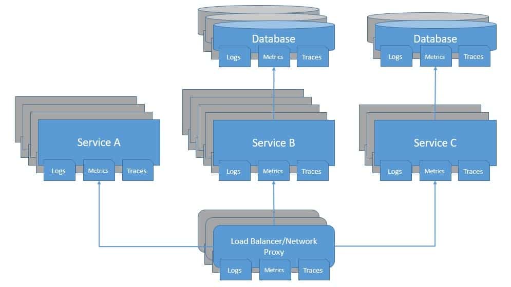
Further, it’s not sufficient just to understand what is happening within applications of a system. For instance, the problem may be in the network layer or the load balancer. Then there are databases, messaging platforms, and the list goes on. It’s important that all these components are observable at all times. We must be able to gather and centralize meaningful data from all parts of the system.
Moreover, since several components are working together, either synchronously or asynchronously, it’s not easy to pinpoint the source of the anomaly. For instance, it’s difficult the say which service in the system is causing the bottleneck escalating as the performance degradation. Traces, as we’ve seen before, are quite useful in investigating such problems.
5. Evolution of Observability
Observability has its roots in control theory, a branch of applied mathematics that deals with the use of feedback to influence the behavior of a system to achieve the desired goal. We can apply this principle in several industries, from industrial plants to aircraft operations. For software systems, this has become popular since some social networking sites like Twitter started to work at massive scales.
Until recent years, most software systems were monolithic, making it fairly easy to reason about them during incidents. Monitoring was quite effective in indicating typical failure scenarios. Further, it was intuitive to debug the code for identifying problems. But, with the advent of microservices architecture and cloud computing, this quickly became a difficult task.
As this evolution continued, software systems were no longer static — they had numerous components that shifted dynamically. This resulted in problems that were never anticipated before. This gave rise to many tools under the umbrella of Application Performance Management (APM), like AppDynamics and Dynatrace. These tools promised a better way to understand the application code and system behavior.
Although these tools have come a long way in evolution, they were fairly metrics-based back then. This prevented them from providing the kind of perspective we required about a systems’ state. However, they were a major step forward. Today, we’ve got a combination of tools to address the three pillars of observability. Of course, the underlying components also need to be observable!
6. Hands-on with Observability
Now that we’ve covered enough theory about observability, let’s see how we can get this into practice. We’ll use a simple microservices-based distributed system where we’ll develop the individual services with Spring Boot in Java. These services will communicate with each other synchronously using the REST APIs.
Let’s have a look at our system services:
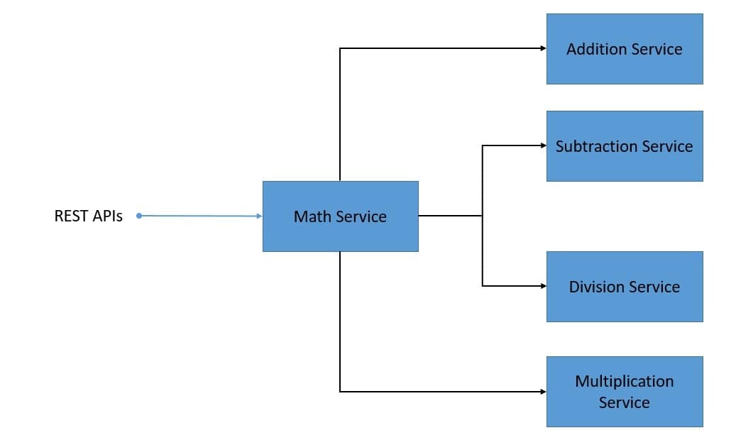
This is a fairly simple distributed system where the math-service uses APIs provided by addition-service, multiplication-service, and others. Further, the math-service exposes APIs to calculate various formulae. We’ll skip the details of creating these microservices as it’s very straightforward.
The emphasis of this exercise is to recognize the most common standards and popular tools available today in the context of observability. Our target architecture for this system with observability will look something like the diagram below:
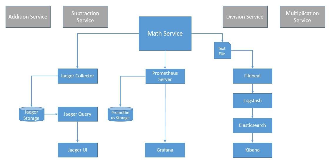
Many of these are also in various stages of recognition with the Cloud Native Computing Foundation (CNCF), an organization that promotes the advancement of container technologies. We’ll see how to use some of these in our distributed system.
7. Traces with OpenTracing
We’ve seen how traces can provide invaluable insights to understand how a single request propagates through a distributed system. OpenTracing is an incubating project under the CNCF. It provides vendor-neutral APIs and instrumentation for distributed tracing. This helps us to add instrumentation to our code that isn’t specific to any vendor.
The list of tracers available that conform to OpenTracing is growing fast. One of the most popular tracers is Jaeger, which is also a graduated-project under the CNCF.
Let’s see how we can use Jaeger with OpenTracing in our application:
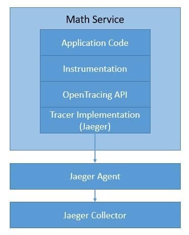
We’ll go through the details later. Just to note, there are several other options like LightStep, Instana, SkyWalking, and Datadog. We can easily switch between these tracers without changing the way we’ve added instrumentation in our code.
7.1. Concepts and Terminology
A trace in OpenTracing is composed of spans. A span is an individual unit of work done in a distributed system. Basically, a trace can be seen as a directed acyclic graph (DAG) of spans. We call the edges between spans as references. Every component in a distributed system adds a span to the trace. Spans contain references to other spans, and this helps a trace to recreate the life of a request.
We can visualize the causal relationship between the spans in a trace with a time-axis or a graph:
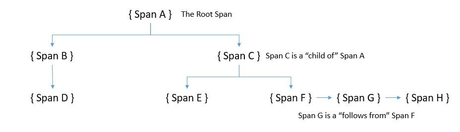
Here, we can see the two types of references that OpenTracing defines, “ChildOf” and “FollowsFrom”. These establish the relationship between the child and the parent spans.
The OpenTracing specification defines the state that a span captures:
- An operation name
- The start time-stamp and the finish time-stamp
- A set of key-value span tags
- A set of key-value span logs
- The SpanContext
Tags allow user-defined annotations to be part of the span we use to query and filter the trace data. Span tags apply to the whole span. Similarly, logs allow a span to capture logging messages and other debugging or informational output from the application. Span logs can apply to a specific moment or event within a span.
Finally, the SpanContext is what ties the spans together. It carries data across the process boundaries. Let’s have a quick look at a typical SpanContext:
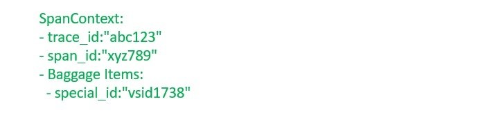
As we can see, it’s primarily comprised of:
- The implementation-dependent state like spanId and traceId
- Any baggage items, which are key-value pairs that cross the process boundary
7.2. Setup and Instrumentation
We’ll begin with installing Jaeger, the OpenTracing compatible tracer that we’ll be using. Although it has several components, we can install them all with a simple Docker command:
docker run -d -p 5775:5775/udp -p 16686:16686 jaegertracing/all-in-one:latestNext, we need to import the necessary dependencies in our application. For a Maven-based application, this is as simple as adding the dependency:
<dependency>
    <groupId>io.opentracing.contrib</groupId>
    <artifactId>opentracing-spring-jaeger-web-starter</artifactId>
    <version>3.3.1</version>
</dependency>
For a Spring Boot-based application, we can leverage this library contributed by third parties. This includes all the necessary dependencies and provides necessary default configurations to instrument web request/response and send traces to Jaeger.
On the application side, we need to create a Tracer:
@Bean
public Tracer getTracer() {
    Configuration.SamplerConfiguration samplerConfig = Configuration
      .SamplerConfiguration.fromEnv()
      .withType("const").withParam(1);
    Configuration.ReporterConfiguration reporterConfig = Configuration
      .ReporterConfiguration.fromEnv()
      .withLogSpans(true);
    Configuration config = new Configuration("math-service")
      .withSampler(samplerConfig)
      .withReporter(reporterConfig);
    return config.getTracer();
}
This is sufficient to generate the spans for the services a request passes through. We can also generate child spans within our service if necessary:
Span span = tracer.buildSpan("my-span").start();
// Some code for which which the span needs to be reported
span.finish();
This is pretty simple and intuitive but extremely powerful when we analyze them for a complex distributed system.
7.3. Trace Analysis
Jaeger comes with a user interface accessible by default at port 16686. It provides a simple way to query, filter, and analyze the trace data with visualization. Let’s see a sample trace for our distributed system:
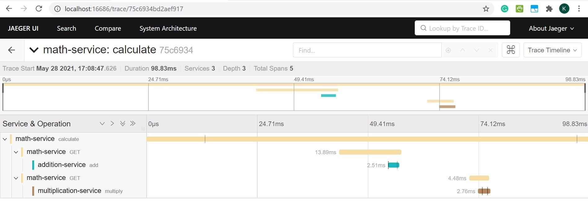
As we can see, this is a visualization for one particular trace identified by its traceId. It clearly shows all the spans within this trace with details like which service it belongs to and the time it took to complete. This can help us understand where the problem may be in the case of atypical behaviors.
8. Metrics with OpenCensus
OpenCensus provides libraries for various languages that allow us to collect metrics and distributed traces from our application. It originated at Google but since then has been developed as an open-source project by a growing community. The benefit of OpenCensus is that it can send the data to any backend for analysis. This allows us to abstract our instrumentation code rather than having it coupled to specific backends.
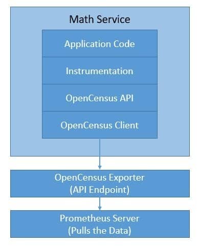
Although OpenCensus can support both traces and metrics, we’ll only use it for metrics in our sample application. There are several backends that we can use. One of the most popular metrics tools is Prometheus, an open-source monitoring solution that is also a graduated-project under the CNCF. Let’s see how Jaeger with OpenCensus integrates with our application:
Although Prometheus comes with a user interface, we can use a visualization tool like Grafana that integrates well with Prometheus.
8.1. Concepts and Terminology
In OpenCensus, a measure represents a metric type to be recorded. For example, the size of the request payload can be one measure to collect. A measurement is a data point produced after recording a quantity by measure. For example, 80 kb can be a measurement for the request payload size measure. All measures are identified by name, description, and unit.
To analyze the stats, we need to aggregate the data with views. Views are basically the coupling of an aggregation applied to a measure and, optionally, tags. OpenCensus supports aggregation methods like count, distribution, sum, and last value. A view is composed of name, description, measure, tag keys, and aggregation. Multiple views can use the same measure with different aggregations.
Tags are key-value pairs of data associated with recorded measurements to provide contextual information and to distinguish and group metrics during analysis. When we aggregate measurements to create metrics, we can use tags as labels to break down the metrics. Tags can also be propagated as request headers in a distributed system.
Finally, an exporter can send the metrics to any backend that is capable of consuming them. The exporter can change depending upon the backend without any impact on the client code. This makes OpenCensus vendor-neutral in terms of metrics collection. There are quite a few exporters available in multiple languages for most of the popular backends like Prometheus.
8.2. Setup and Instrumentation
Since we’ll be using Prometheus as our backend, we should begin by installing it. This is quick and simple using the official Docker image. Prometheus collects metrics from monitored targets by scraping metrics endpoints on these targets. So, we need to provide the details in the Prometheus configuration YAML file, prometheus.yml:
scrape_configs:
  - job_name: 'spring_opencensus'
    scrape_interval: 10s
    static_configs:
      - targets: ['localhost:8887', 'localhost:8888', 'localhost:8889']
This is a fundamental configuration that tells Prometheus which targets to scrape metrics from. Now, we can start Prometheus with a simple command:
docker run -d -p 9090:9090 -v \
  ./prometheus.yml:/etc/prometheus/prometheus.yml prom/prometheus
For defining custom metrics, we begin by defining a measure:
MeasureDouble M_LATENCY_MS = MeasureDouble
  .create("math-service/latency", "The latency in milliseconds", "ms");
Next, we need to record a measurement for the measure we’ve just defined:
StatsRecorder STATS_RECORDER = Stats.getStatsRecorder();
STATS_RECORDER.newMeasureMap()
  .put(M_LATENCY_MS, 17.0)
  .record();
Then, we need to define an aggregation and view for our measure that will enable us to export this as a metric:
Aggregation latencyDistribution = Distribution.create(BucketBoundaries.create(
  Arrays.asList(0.0, 25.0, 100.0, 200.0, 400.0, 800.0, 10000.0)));
View view = View.create(
  Name.create("math-service/latency"),
  "The distribution of the latencies",
  M_LATENCY_MS,
  latencyDistribution,
  Collections.singletonList(KEY_METHOD)),
};
ViewManager manager = Stats.getViewManager();
manager.registerView(view);
Finally, for exporting views to Prometheus, we need to create and register the collector and run an HTTP server as a daemon:
PrometheusStatsCollector.createAndRegister();
HTTPServer server = new HTTPServer("localhost", 8887, true);
This is a straightforward example that illustrates how we can record latency as a measure from our application and export that as a view to Prometheus for storage and analysis.
8.3. Metrics Analysis
OpenCensus provides in-process web pages called zPages that display collected data from the process they’re attached to. Further, Prometheus offers the expressions browser that allows us to enter any expression and see its result. However, tools like Grafana provide a more elegant and efficient visualization.
Installing Grafana using the official Docker image is quite simple:
docker run -d --name=grafana -p 3000:3000 grafana/grafanaGrafana supports querying Prometheus — we simply need to add Prometheus as a data source in Grafana. Then, we can create a graph with a regular Prometheus query expression for metrics:
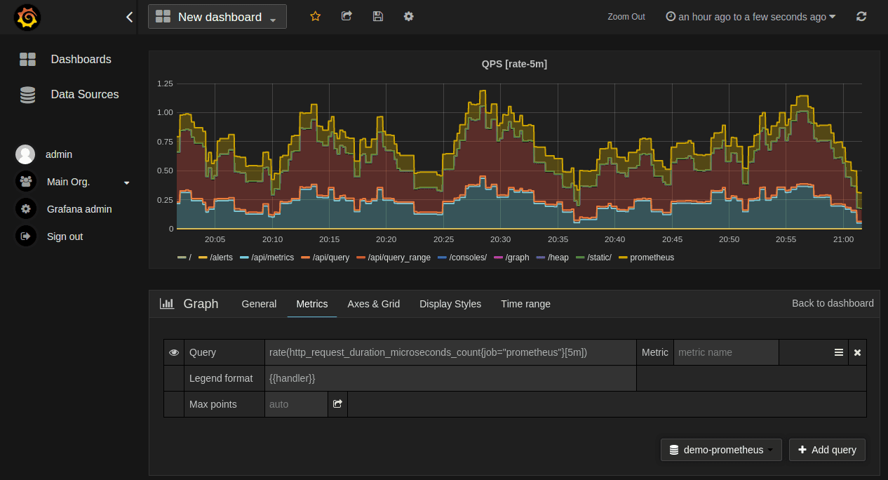
There are several graph settings that we can use to tune our graph. Additionally, there are several pre-built Grafana dashboards available for Prometheus that we may find useful.
9. Logs with Elastic Stack
Logs can provide invaluable insights into the way an application reacted to an event. Unfortunately, in a distributed system, this is split across multiple components. Hence, it becomes important to collect logs from all the components and store them in one single place for effective analysis. Moreover, we require an intuitive user interface to efficiently query, filter and reference the logs.
Elastic Stack is basically a log management platform that, until recently, was a collection of three products – Elasticsearch, Logstash, and Kibana (ELK).
However, since then, Beats have been added to this stack for efficient data collection.
Let’s see how we can use these products in our application:
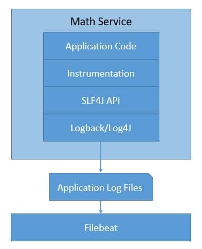
As we can see, in Java, we can generate logs with a simple abstraction like SLF4J and a logger like Logback. We will skip these details here.
The Elastic Stack products are open-source and maintained by Elastic. Together, these provide a compelling platform for log analysis in a distributed system.
9.1. Concepts and Terminology
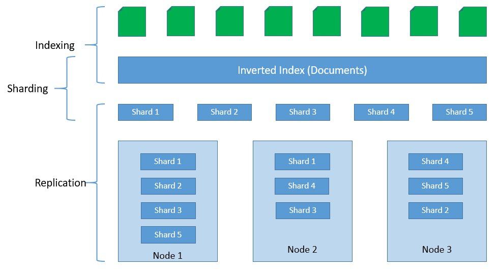
As we’ve seen, Elastic Stack is a collection of multiple products. The earliest of these products was Elasticseach, which is a distributed, RESTful, JSON-based search engine. It’s quite popular due to its flexibility and scalability. This is the product that led to the foundation of Elastic. It’s fundamentally based on the Apache Lucene search engine.
Elasticsearch stores indices as documents, which are the base unit of storage. These are simple JSON objects. We can use types to subdivide similar types of data inside a document. Indices are the logical partitions of documents. Typically, we can split indices horizontally into shards for scalability. Further, we can also replicate shards for fault tolerance:
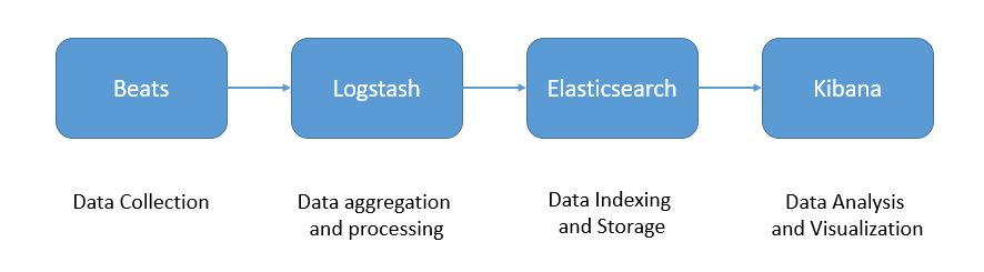
Logstash is a log aggregator that collects data from various input sources It also executes different transformations and enhancements and ships it to an output destination. Since Logstash has a larger footprint, we have Beats, which are lightweight data shippers that we can install as agents on our servers. Finally, Kibana is a visualization layer that works on top of Elasticsearch.
Together, these products offer a complete suite to perform aggregation, processing, storage, and analysis of the log data:
With these products, we can create a production-grade data pipeline for our log data. However, it’s quite possible, and in some cases also necessary, to extend this architecture to handle large volumes of log data. We can place a buffer like Kafka in front of Logstash to prevent downstream components from overwhelming it. Elastic Stack is quite flexible in that regard.
9.2. Setup and Instrumentation
The Elastic Stack, as we’ve seen earlier, comprises several products. We can, of course, install them independently. However, that is time-consuming. Fortunately, Elastic provides official Docker images to make this easy.
Starting a single-node Elasticsearch cluster is as simple as running a Docker command:
docker run -p 9200:9200 -p 9300:9300 \
  -e "discovery.type=single-node" \
  docker.elastic.co/elasticsearch/elasticsearch:7.13.0
Similarly, installing Kibana and connecting it to the Elasticsearch cluster is quite easy:
docker run -p 5601:5601 \
  -e "ELASTICSEARCH_HOSTS=http://localhost:9200" \
  docker.elastic.co/kibana/kibana:7.13.0
Installing and configuring Logstash is a little more involved as we have to provide the necessary settings and pipeline for data processing. One of the simpler ways to achieve this is by creating a custom image on top of the official image:
FROM docker.elastic.co/logstash/logstash:7.13.0
RUN rm -f /usr/share/logstash/pipeline/logstash.conf
ADD pipeline/ /usr/share/logstash/pipeline/
ADD config/ /usr/share/logstash/config/
Let’s see a sample configuration file for Logstash that integrates with Elasticsearch and Beats:
input {
  tcp {
  port => 4560
  codec => json_lines
  }
  beats {
    host => "127.0.0.1"
    port => "5044"
  }
}
output{
  elasticsearch {
  hosts => ["localhost:9200"]
  index => "app-%{+YYYY.MM.dd}"
  document_type => "%{[@metadata][type]}"
  }
  stdout { codec => rubydebug }
}
There are several types of Beats available depending upon the data source. For our example, we’ll be using the Filebeat. Installing and configuring Beats can be best done with the help of a custom image:
FROM docker.elastic.co/beats/filebeat:7.13.0
COPY filebeat.yml /usr/share/filebeat/filebeat.yml
USER root
RUN chown root:filebeat /usr/share/filebeat/filebeat.yml
USER filebeat
Let’s look at a sample filebeat.yml for a Spring Boot application:
filebeat.inputs:
- type: log
enabled: true
paths:
  - /tmp/math-service.log
output.logstash:
hosts: ["localhost:5044"]
This is a very cursory but complete explanation of the installation and configuration for the Elastic Stack. It’s beyond the scope of this tutorial to go into all the details.
9.3. Log Analysis
Kibana provides a very intuitive and powerful visualization tool for our logs. We can access the Kibana interface at its default URL, http://localhost:5601. We can select a visualization and create a dashboard for our application.
Let’s see a sample dashboard:
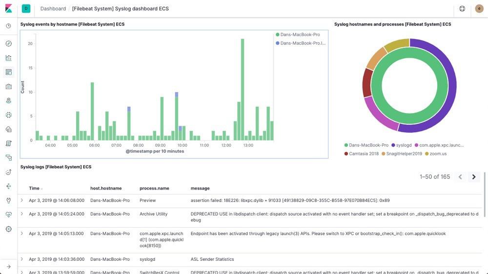
Kibana offers quite extensive capabilities to query and filter the log data. These are beyond the scope of this tutorial.
10. The Future of Observability
Now, we’ve seen why observability is a key concern for distributed systems. We’ve also gone through some of the popular options for handling different types of telemetry data that can enable us to achieve observability. However, the fact remains, it’s still quite complex and time-consuming to assemble all the pieces. We have to handle a lot of different products.
One of the key advancements in this area is OpenTelemetry, a sandbox project in the CNCF. Basically, OpenTelemetry has been formed through a careful merger of OpenTracing and OpenCensus projects. Obviously, this makes sense as we’ll only have to deal with a single abstraction for both traces and metrics.
What’s more, OpenTelemetry has a plan to support logs and make them a complete observability framework for distributed systems. Further, OpenTelemetry has support for several languages and integrates well with popular frameworks and libraries. Also, OpenTelemetry is backward compatible with OpenTracing and OpenCensus via software bridges.
OpenTelemetry is still in progress, and we can expect this to mature in the coming days. Meanwhile, to ease our pain, several observability platforms combine many of the products discussed earlier to offer a seamless experience. For instance, Logz.io combines the power of ELK, Prometheus, and Jaeger to offer a scalable platform as a service.
The observability space is fast maturing with new products coming into the market with innovative solutions. For instance, Micrometer provides a vendor-neutral facade over the instrumentation clients for several monitoring systems. Recently, OpenMetrics has released its specification for creating a de facto standard for transmitting cloud-native metrics at scale.
11. Conclusion
In this tutorial, we went through the basics of observability and its implications in a distributed system. We also implemented some of the popular options today for achieving observability in a simple distributed system.
This allowed us to understand how OpenTracing, OpenCensus, and ELK can help us build an observable software system. Finally, we discussed some of the new developments in this area and how we can expect observability to grow and mature in the future.