

Yes, we're now running our only Summer Sale. All Courses are 30% off until 20th July, 2026:
Learn through the super-clean Baeldung Pro experience:
>> Membership and Baeldung Pro.
No ads, dark-mode and 6 months free of IntelliJ Idea Ultimate to start with.
1. Introduction
In Natural Language Processing, we want computers to understand the text as we humans do. However, for this to happen, we need them to translate the words to a language computers can work with and understand.
In this tutorial, we’ll discuss how to achieve this by using word embeddings. We’ll examine what they are and why they are important.
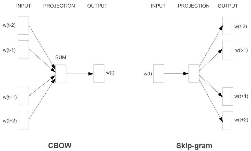
We’ll also present the two main methods to obtain word embeddings: CBOW and Skip-Gram.
2. Word Embeddings
What is word embedding? Word embedding is a numerical representation of words, such as how colors can be represented using the RGB system.
A common representation is one-hot encoding. This method encodes each word with a different vector. The size of the vectors equals the number of words. Thus, if there are  words, the vectors have a size of
  . All values in the vectors are zeros except for a value 1, which differentiates each word representation.
Let’s use the following sentence, the pink horse is eating. In this example, there are  words; therefore, the size of the vectors is
  . Let’s see how it works:
![\[ \text{\huge{ the pink horse is eating }} \]](/wp-content/ql-cache/quicklatex.com-40dd0ac8f7ba6930347fc88ac01ef5b8_l3.svg "Rendered by QuickLaTeX.com")
![\[ \text{\huge{the}} \rightarrow \begin{bmatrix} 1 \\ 0 \\ 0 \\ 0 \\ 0 \end{bmatrix} \hspace{1cm} \text{\huge{pink}} \rightarrow \begin{bmatrix} 0 \\ 1 \\ 0 \\ 0 \\ 0 \end{bmatrix} \hspace{1cm} \text{\huge{horse}} \rightarrow \begin{bmatrix} 0 \\ 0 \\ 1 \\ 0 \\ 0 \end{bmatrix} \hspace{1cm} \text{\huge{is}} \rightarrow \begin{bmatrix} 0 \\ 0 \\ 0 \\ 1 \\ 0 \end{bmatrix} \hspace{1cm} \text{\huge{eating}} \rightarrow \begin{bmatrix} 0 \\ 0 \\ 0 \\ 0 \\ 1 \end{bmatrix} \]](/wp-content/ql-cache/quicklatex.com-aca3b72bad8941a430b71c9946bf01b3_l3.svg "Rendered by QuickLaTeX.com")
Each word gets assigned a different vector; however, this representation involves different issues. First of all, if the vocabulary is too big, the size of the vectors will be huge. This would lead to the curse of dimensionality when using a model with this encoding. Also, if we add or remove words to the vocabulary, the representation of all words will change.
However, the most important problem of using one-hot encoding is that it doesn’t encapsulate meaning. It is just a numeration system to distinguish words. If we want computers to read text as humans do, we need embeddings that capture semantic and syntactic information. The values in the vectors must somehow quantify the meaning of the words they represent.
Word2Vec is a common technique used in Natural Language Processing. In it, similar words have similar word embeddings; this means that they are close to each other in terms of cosine distance. There are two main algorithms to obtain a Word2Vec implementation: Continous Bag of Words and Skip-Gram. These algorithms use neural network models in order to obtain the word vectors.
These models work using context. This means that the embedding is learned by looking at nearby words; if a group of words is always found close to the same words, they will end up having similar embeddings. Thus, countries will be closely related, so will animals, and so on.
To label how words are close to each other, we first set a window-size. The window-size determines which nearby words we pick. For example, given a window-size of 2, for every word, we’ll pick the 2 words behind it and the 2 words after it:
| Sentence | Word pairs |
|---|---|
| the pink horse is eating | (the, pink), (the, horse) |
| the pink horse is eating | (pink, the), (pink, horse), (pink, is) |
| the pink horse is eating | (horse, the), (horse, pink), (horse, is), (horse, eating) |
| the pink horse is eating | (is, pink), (is, horse), (is, eating) |
| the pink horse is eating | (eating, horse), (eating, is) |
In the table above, we can see the word pairs constructed with this method. The highlighted word is the one we are finding pairs for. We don’t care about how far the words in the window are. We don’t differentiate between words that are 1 word away or more, as long as they’re inside the window.
Now that we know how to find the word pairs, let’s find out how these algorithms work.
3. Skip-Gram
As previously mentioned, both algorithms use nearby words in order to extract the semantics of the words into embeddings. In Skip-Gram, we try to predict the context words using the main word.
Let’s use the previous example. From the sentence the pink horse is eating, let’s say we want to get the embedding for the word horse. First, we encode all words in the corpus to train by using one-hot encoding. We pick the word pairs of the word we want to find the embedding of: (horse, the), (horse, pink), (horse, is), (horse, eating). Now from each of them, we use a Neural Network model with one hidden layer, as represented in the following image:
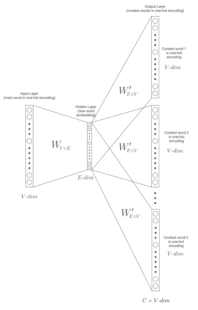
In the picture, we can see the input layer with a size of  , where
  is the number of words in the corpus vocabulary. The input is the main word in one-hot encoding, horse in our example. The weight matrix
  transforms the input into the hidden layer.
This hidden layer has a size of  , where
  is the desired size of the word embeddings. The higher this size is, the more information the embeddings will capture, but the harder it will be to learn it.
Finally, the weight matrix  transforms the hidden layer into the output layer. As the outputs to be predicted are going to be the context words in one-hot encoding, the final layer will have a size of . We’ll run the model once per context word. The model will learn by trying to predict the context words.
Once the training is done in the whole vocabulary, we’ll have a weight matrix  of size
  that connects the input to the hidden layer. With it, the embeddings can now be obtained. If it has been done correctly, the representation encapsulates semantics, as we mentioned before, and similar words are close to each other in the vectorial world.
4. CBOW
In Continuous Bag of Words, the algorithm is really similar, but doing the opposite operation. From the context words, we want our model to predict the main word:
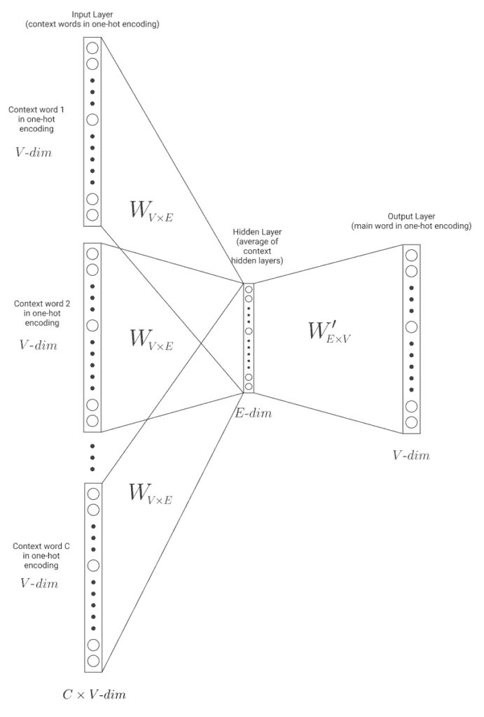
As in Skip-Gram, we have the input layer (which now consists of the context words in one-hot encoding – size ). For every context word, we get the hidden layer resulting from the weight matrix . Then we average them into a single hidden layer, which is passed on to the output layer. The model learns to predict the main word, tweaking the weight matrixes.
Again, once the training is done, we use the weight matrix to generate the word embeddings from the one-hot encodings.
5. CBOW vs Skip-Gram
Now that we have a broad idea of both models, which one is better? As is usually the case, it depends:
According to the original paper, Mikolov et al., it is found that Skip-Gram works well with small datasets, and can better represent less frequent words.
However, CBOW is found to train faster than Skip-Gram, and can better represent more frequent words.
Of course, which model we choose largely depends on the problem we’re trying to solve. Is it important for our model to represent rare words? If so, we should choose Skip-Gram. We don’t have much time to train and rare words are not that important for our solution? Then we should choose CBOW.
6. Conclusion
In this article, we learned what word embeddings are and why we use them in NLP. We then presented one-hot encoding, a simple embedding that doesn’t take into account the semantics of the words.
Next, we examined CBOW and Skip-Gram, two algorithms that, from this encoding, are able to produce a transformation in order to obtain embeddings that encapsulate syntactic and semantic information from the words.
Finally, we discussed how these algorithms differ, and which one would be more useful depending on the problem to be solved.