When Coherence Score Is Good or Bad in Topic Modeling?

1. Introduction

In this tutorial, we’ll explain one of the most challenging natural language processing area known as topic modeling. We can use topic modeling for recognizing and extracting different topics from the text. It helps us easily understand the information from a large amount of textual data. After the introduction, we’ll dive deeper into understanding the related concepts, such as LDA and coherence score. The whole accent will be towards getting familiar with these measurements and how to interpret their values.

2. Topic Modeling

Topic modeling is a machine learning and natural language processing technique for determining the topics present in a document. It’s capable of determining the probability of a word or phrase belonging to a certain topic and cluster documents based on their similarity or closeness. It does this by analyzing the frequency of words and phrases in the documents. Some applications of topic modeling also include text summarization, recommender systems, spam filters, and similar.

Specifically, the current methods for extraction of topic models include Latent Dirichlet Allocation (LDA), Latent Semantic Analysis (LSA), Probabilistic Latent Semantic Analysis (PLSA), and Non-Negative Matrix Factorization (NMF). We’ll focus on the coherence score from Latent Dirichlet Allocation (LDA).

3. Latent Dirichlet Allocation (LDA)

Latent Dirichlet Allocation is an unsupervised, machine learning, clustering technique that we commonly use for text analysis. It’s a type of topic modeling in which words are represented as topics, and documents are represented as a collection of these word topics.

In summary, this method recognizes topics in the documents through several steps:

Sampling topics – initialize the Dirichlet distribution of documents in the topic’s space and choose $N$ topics from multinomial distribution of topics over a document.
Sampling words and creating a document – initialize the Dirichlet distribution of topics in the word’s space and choose $N$ words, for each of the previously sampled topics, from the multinomial distribution of words over topics.
Maximize the probability of creating the same documents.

Following that, the algorithm above is mathematically defined as

(1) $\begin{equation*} P(\boldsymbol{W}, \boldsymbol{Z}, \boldsymbol{\theta}, \boldsymbol{\phi}; \alpha, \beta) = \prod_{i = 1}^{M}P(\theta_{j}; \alpha)\prod_{i = 1}^{K}P(\phi; \beta)\prod_{t = 1}^{N}P(Z_{j, t} | \theta_{j})P(W_{j, t} | \phi z_{j, t}), \end{equation*}$

where $\alpha$ and $\beta$ define Dirichlet distributions, $\theta$ and $\phi$ define multinomial distributions, $\bold{Z}$ is the vector with topics of all words in all documents, $\bold{W}$ is the vector with all words in all documents, $M$ number of documents, $K$ number of topics and $N$ number of words.

We can do the whole process of training or maximizing probability using Gibbs sampling, where the general idea is to make each document and each word as monochromatic as possible. Basically, it means we want that each document to have as few as possible articles, and each word belongs to as few as possible topics.

4. Coherence Score

We can use the coherence score in topic modeling to measure how interpretable the topics are to humans. In this case, topics are represented as the top N words with the highest probability of belonging to that particular topic. Briefly, the coherence score measures how similar these words are to each other.

4.1. CV Coherence Score

One of the most popular coherence metrics is called CV. It creates content vectors of words using their co-occurrences and, after that, calculates the score using normalized pointwise mutual information (NPMI) and the cosine similarity. This metric is popular because it’s the default metric in the Gensim topic coherence pipeline module, but it has some issues. Even the author of this metric doesn’t recommend using it.

Because of that, we don’t recommend using the CV coherence metric.

4.2. UMass Coherence Score

Instead of using the CV score, we recommend using the UMass coherence score. It calculates how often two words, $w_{i}$ and $w_{j}$ appear together in the corpus and it’s defined as

(2) $\begin{equation*} C_{UMass}(w_{i}, w_{j}) = \log \frac{D(w_{i}, w_{j}) + 1}{D(w_{i})}, \end{equation*}$

where $D(w_{i}, w_{j})$ indicates how many times words $w_{i}$ and $w_{j}$ appear together in documents, and $D(w_{i})$ is how many time word $w_{i}$ appeared alone. The greater the number, the better is coherence score. Also, this measure isn’t symmetric, which means that $C_{UMass}(w_{i}, w_{j})$ is not equal to $C_{UMass}(w_{j}, w_{i})$ . We calculate the global coherence of the topic as the average pairwise coherence scores on the top $N$ words which describe the topic.

4.3. UCI Coherence Score

This coherence score is based on sliding windows and the pointwise mutual information of all word pairs using top $N$ words by occurrence. Instead of calculating how often two words appear in the document, we calculate the word co-occurrence using a sliding window. It means that if our sliding window has a size of 10, for one particular word $w_{i}$ , we observe only 10 words before and after the word $w_{i}$ .

Therefore, if both words $w_{i}$ and $w_{j}$ appeared in the document but they’re not together in one sliding window, we don’t count as they appeared together. Similarly, as for the UMass score, we define the UCI coherence between words $w_{i}$ and $w_{j}$ as

(3) $\begin{equation*} C_{UCI}(w_{i}, w_{j}) = \log \frac{P(w_{i}, w_{j}) + 1}{P(w_{i}) \cdot P(w_{j})}. \end{equation*}$

where $P(w)$ is probability of seeing word $w$ in the sliding window and $P(w_{i}, w_{j})$ is probability of appearing words $w_{i}$ and $w_{j}$ together in the sliding window. In the original paper, those probabilities were estimated from the entire corpus of over two million English Wikipedia articles using a 10-words sliding window. We calculate the global coherence of the topic in the same way as for the UMass coherence.

4.4. Word2vec Coherence Score

One smart idea is to utilize the word2vec model for the coherence score. This will introduce the semantic of the words in our score. Basically, we want to measure our coherence based on two criteria:

Intra-topic similarity – the similarity of words in the same topic.
Inter-topic similarity – the similarity of words across different topics.

The idea is pretty simple. We want to maximize intra-topic and minimize inter-topic similarity. Also, by similarity, we imply the cosine similarity between words represented by word2vec embedding.

Following that, we compute intra-topic similarity per topic as an average similarity between every possible pair of top $N$ words in that topic. Consequently, we compute the inter-topic similarity between two topics as an average similarity between top $N$ words from these topics.

Finally, the word2vec coherence score between two topics, $t_{i}$ and $t_{j}$ , is calculated as

(4) $\begin{equation*} C_{word2vec}(t_{i}, t_{j}) = \frac{\frac{intra\_topic\_similarity(t_{i}) + intra\_topic\_similarity(t_{j})}{2}}{inter\_topic\_similarity(t_{i}, t_{j})}. \end{equation*}$

4.5. Choosing the Best Coherence Score

There is no one way to determine whether the coherence score is good or bad. The score and its value depend on the data that it’s calculated from. For instance, in one case, the score of 0.5 might be good enough but in another case not acceptable. The only rule is that we want to maximize this score.

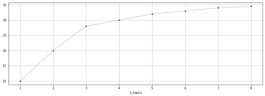
Usually, the coherence score will increase with the increase in the number of topics. This increase will become smaller as the number of topics gets higher. The trade-off between the number of topics and coherence score can be achieved using the so-called elbow technique. The method implies plotting coherence score as a function of the number of topics. We use the elbow of the curve to select the number of topics.

The idea behind this method is that we want to choose a point after which the diminishing increase of coherence score is no longer worth the additional increase of the number of topics. The example of elbow cutoff at $n\_topics = 3$ is shown below:

Also, the coherence score depends on the LDA hyperparameters, such as $\alpha$ , $\beta$ , and $K$ . Because of that, we can use any machine learning hyperparameter tuning technique. After all, it’s important to manually validate results because, in general, the validation of unsupervised machine learning systems is always a tricky task.

5. Conclusion

In this article, we introduced the intuition behind the topic modeling concept. Also, we explained in detail the LDA algorithm that is one of the most popular methods for solving this task. In the end, we resolve the problem of determining the meaning of the coherence score and how to know when this score is good or bad.

Generally, the topic modeling task is one of the most challenging tasks in natural language processing. There is a lot of research around this concept, and the interest will only grow because of the increasing amount of textual data on the internet.

Full Archive

About Baeldung

Core Concepts

Operating Systems

Artificial Intelligence

Graph Theory

Latex