

Learn through the super-clean Baeldung Pro experience:
>> Membership and Baeldung Pro.
No ads, dark-mode and 6 months free of IntelliJ Idea Ultimate to start with.
Learn through the super-clean Baeldung Pro experience:
>> Membership and Baeldung Pro.
No ads, dark-mode and 6 months free of IntelliJ Idea Ultimate to start with.
A self-organizing map (SOM) is a special type of neural network we use for reducing the dimensionality of high-dimensional data.
SOMs belong to unsupervised algorithms such as principal component analysis (PCA) and k-means clustering and are also called Kohonen maps or networks after their inventor, Teuvo Kohonen.
In this tutorial, we’ll learn about the motivation behind this algorithm, its procedure, and its applications.
Most of the time, our data are high-dimensional. That makes them difficult to analyze and extract useful patterns from them. In such cases, we usually apply unsupervised learning algorithms for dimensionality reduction, e.g., k-means.
K-means breaks the data into a predefined number of clusters ( ) and assigns each data point to one of them. However, we must use the correct number of clusters for k-means to work. Finding the number can be tricky and require multiple guesses and runs, which takes time.
A better way would be to devise an algorithm that can guess the correct number of clusters on its own. This is where self-organizing maps come to the rescue. As we’ll see in the next section, a SOM is a lattice of neurons. Its size depends on the application.
A SOM is a single-layer neural network. Its neurons are in a  lattice (we choose the values of and
  ):
):
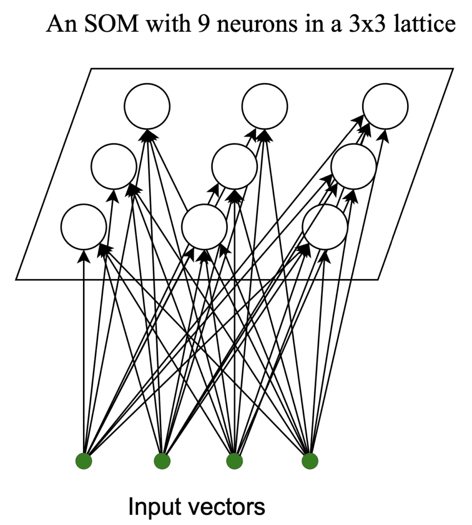
The neurons in the lattice are vectors we initialize randomly and train using competitive learning. There’s no hard and fast rule for determining the lattice size. However, as a rule of thumb, we can use  neurons, where
  is the number of data points in the training set. This is usually large enough to capture the dominant patterns in the data.
In the case of clustering, for instance, similar data points will make specific regions of neurons denser and thus form clusters. Other regions, on the other hand, will become shallower.
SOMs iteratively run three stages until convergence: competition, cooperation, and adaptation.
In this stage, we go over all the input data points. Then, for each, we measure the distance between its vector and each neuron in the lattice (e.g., Euclidean distance).
After calculating the distances, we find the neuron closest to the input vector neuron. This stage is called competition because the neurons compete in similarity to our data point.
The cooperation phase begins after finding the winning neuron. In it, we find the winning neuron’s neighbors.
The neighborhood is defined through the neighborhood function  . It quantifies the degree to which a neuron can be considered a neighbor of the winning neuron. While doing so, follows two rules:
Here, we update the neurons according to  :
:
![\[ w_{j}(n+1) = w_{j}(n) + \alpha h_{ij} \Bigl( d\left(x, w_{j}(n)\right) \Bigr)\]](/wp-content/ql-cache/quicklatex.com-f4a531562df1765505292408a8609ef2_l3.svg "Rendered by QuickLaTeX.com")
where:
 is the input vector
 is the vector representation of neuron
  at iteration
  (
( is the winning neuron)
 is the learning rate
 is a distance function
For instance, we can use the Gaussian function to focus the winner’s influence on the neurons close to it:
![\[ h(d(i, j)) = e^{-\frac{d^2(i, j)}{2\sigma^2}}\]](/wp-content/ql-cache/quicklatex.com-e5b4364a982c308a7de0fff818a5e35c_l3.svg "Rendered by QuickLaTeX.com")
where  is the Euclidean distance between neighbor and the winning neuron
  , and
, and  is the standard deviation of the Gaussian function.
In some variations of the algorithm, decreases with time.
In addition to the training data, the algorithm also requires several hyperparameters, such as the size of lattice  , the neighborhood function , and the number of iterations
  :
:
algorithm SOM(X, k, l, h, M):
    // INPUT
    //    X = training data
    //    k = the number of rows in the lattice
    //    l = the number of columns in the lattice
    //    M = the maximal number of iterations
    //    h = the neighborhood function
    // OUTPUT
    //    V = SOM vectors

    Randomly initialize SOM vectors V

    for n <- 1 to M:
        for sample in X:
            // competition
            Find the neuron closest to the sample

            // cooperation and adaptation
            Update V with respect to the winning neuron

    return V
Convergence occurs when there’s no noticeable change in the map. In other words, if new inputs map to the same neurons from the previous iteration, the network has converged to a solution.
The cooperation and adaptation stages are intertwined. Therefore, we can consider them one phase in the computational sense.
SOMs and K-means can both be used for clustering the data. However, we can think of SOMs as a constrained version of K-means. This means that the neurons in SOMs aren’t as free to move as the centroids in K-means are.
However, in K-means, we have to specify the number of clusters beforehand, while SOMs don’t need that. The reason is that the initial lattice that we choose can be large, allowing neurons to cluster on their own. We can see this in a diagram of how SOMs work:
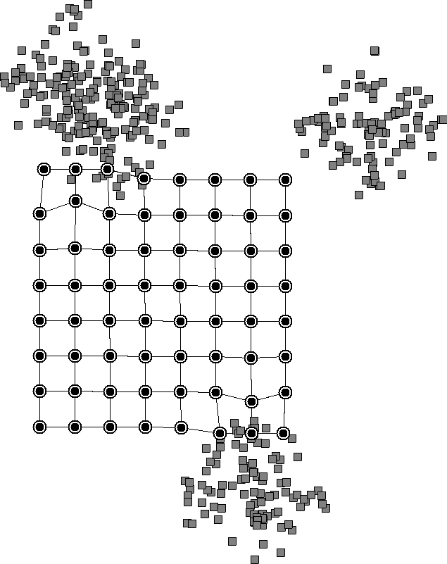
The nearby neurons move together and reveal clusters in the data. We don’t need to specify the number of clusters beforehand since the neurons will learn it from the data.
Another drawback of K-means is that it can be more sensitive to outliers since they can move the centroids toward themselves, away from the clusters in the data. This is not the case with SOMs.
Finally, SOMs keep the topological structure of the data, whereas K-means doesn’t. This is because, in K-means, each centroid moves freely without regard for the others. However, in SOMs, the shift in a neuron’s place is relative to the winning neuron. As a result, SOMs keep the underlying topology of the data, which is shown in the above diagram.
In this article, we learned about self-organizing maps (SOMs). We can use them to reduce data dimensionality and visualize the data structure while preserving its topology.