The Skip List Data Structure | Baeldung on Computer Science

1. Introduction

In this tutorial, we’ll talk about skip lists. They are a popular probabilistic alternative to balanced trees. We’ll explain how the skip lists work and show how to implement three standard operations on them: insertion, search, and deletion.

2. Motivation

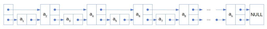
Let’s imagine a sorted linked list with $n$ numbers:

If we search for a number in it, we’ll traverse all $n$ elements in the worst case (when the sought value is greater than the list’s maximum). We start from the first node and follow all the pointers to the last one.

Now, let’s add a pointer two nodes ahead to every other node:

Starting from the first node, we can skip two nodes at a time, so we won’t visit more than $\approx n/2$ nodes in the worst case before we either find the number we seek or conclude it’s not in the list:

What would happen if we gave every fourth node a pointer four nodes ahead of it? Then, the number of nodes we visit in the worst case would be approximately $n / 4$ . In general, if every $\boldsymbol{2^k}$ -th node has a pointer to the node $\boldsymbol{2^k}$ nodes ahead of it, we reduce the number of nodes we have to examine in the worst-case search scenario to $\boldsymbol{O(\log n)}$ .

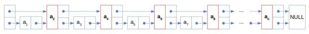
That’s the main idea behind skip lists. They contain nodes with more than one forward pointer, thus allowing for fast lookup. A node with $k$ forward pointers is called a level- $k$ node. Half the nodes are level 1, $25\%=1/(2^2)$ of the nodes are level 2, $25\%=1/(2^3)$ are level 3, $1/(2^{k})$ nodes are level $k$ , and so on.

3. Skip Lists as Probabilistic Structures

However, deletion and insertion would be impractical in the case of the above skip list. After deleting or inserting an element, we’ll have to update the pointers to keep pointing to the new nodes at appropriate positions.

A way to avoid the overhead is to keep the changes local. We can do that if we don’t fix the positions of the higher-level nodes. For example, we can decide the level of a new node randomly so that higher-level nodes aren’t necessarily $2^k$ ( $k > 1$ ) nodes from one another. Instead, a level- $k$ pointer will point to the next level- $k$ node wherever it is in the list. That way, insertions, and deletions won’t lead to rearranging the pointers other than that pointed to the node immediately after the inserted one. The analogous reasoning holds for deletion.

To keep the logarithmic complexity of the search, we can maintain the same ratio of the levels’ sizes from the above example. We do that by setting to $1/2$ the probability to advance a level-( $k-1$ ) node to the level $k$ while inserting it into the list. In that case, we’ll have approximately $1/(2^{k})$ nodes at level $k \geq 1$ .

Therefore, a skip list is a multilevel linked list with its nodes’ levels decided randomly.

3.1. How to Set the Levels

If we don’t limit the levels in advance, they’ll depend only on the chosen chance to advance a node during insertion. We don’t have to use $1/2$ as in the above example. Any $\boldsymbol{p \in (0, 1)}$ can serve as the probability, and the time complexity of search will still be $\boldsymbol{O(\log n)}$ .

Here’s the pseudocode for selecting a new node’s level:

3.2. The Expected Level

A node cannot be at the level $k > 1$ without first becoming a level- $(k-1)$ node. So, the probability of a node being at level $\boldsymbol{k>1}$ is $\boldsymbol{p^{k-1}(1-p)}$ (we subtract 1 because we don’t toss the dice for deciding the first level). From there, we see that a node’s level minus 1 follows a geometric distribution with $1-p$ as the “success probability”. So, the expected value of a node’s level is:

(1)

3.3. The Number of Pointers

There are $n$ pointers in a single-linked list with $n$ nodes. One of them points to the head, while the rest form the links between the nodes. Since all the nodes’ levels are $\geq 1$ , we know there will be $n$ level-1 pointers.

At the second level, we expect to have $p(1-p)n$ pointers, the same as the expected number of level-2 nodes. The same applies to the higher levels. So, the expected number of pointers is (if $maxLevel$ is $\infty$ ):

$\begin{aligned} n + \sum_{k=2}^{\infty}p^{k-1}(1-p)n &= n \left(1 +\sum_{k=2}^{\infty}p^{k-1}(1-p) \right) \\ &= n \left( 1 + (1-p)\sum_{k-1}^{\infty}p^k \right) \\ &= n \left( 1 + (1-p)\frac{p}{1-p} \right) \\ &= n \left( 1 + p ) \end{aligned}$

With the maximal level set to $L<\infty$ , the number of pointers is bounded from above by $n(1+p)$ . Since $p$ is independent of $n$ , the expected memory complexity of a skip list is $\boldsymbol{O(n)}$ , same as the space complexity of a linked list. Moreover, we see that we won’t ever use more than twice the pointers a single-linked list has (since $p \leq 1$ ).

3.4. The Infrastructure

We’ll consider a node the data structure with the following attributes:

$value$ : the value it contains
$successors$ : the array of pointers to the successors at various levels

Similarly, we’ll assume that the list is a data structure with two attributes:

$maxLevel$ – the current maximal level of the list
$heads$ – the array of pointers to the heads at the levels $1,2, \ldots, list.maxLevel$

4. How to Insert Into a Skip List

To insert a node with value $v$ into a skip list, we have to do three things:

find where to place it
choose its level
and update the pointer that should point to the new node

We’ve already seen how to choose the level $\ell$ of the new node $y$ . To find where to place it, we start from the head node at the top level and follow the pointers until we reach two consecutive nodes, $\boldsymbol{x}$ and $\boldsymbol{z}$ , such that $\boldsymbol{x.value < v \leq z.value}$ . If such nodes exist and $\ell$ isn’t greater than the current level (i.e., the top-level), we should update $x$ to point to $y$ and set the new node to point to $z$ . Then, we repeat the steps until we reach the bottom layer.

If the new node’s level is higher than the current maximal level of the entire list, we should insert new levels. We do that by setting the new node as their head.

4.1. Pseudocode

Here’s the pseudocode of insertion:

4.2. Example

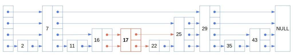
Let’s say that we want to insert the number $17$ into this skip list:

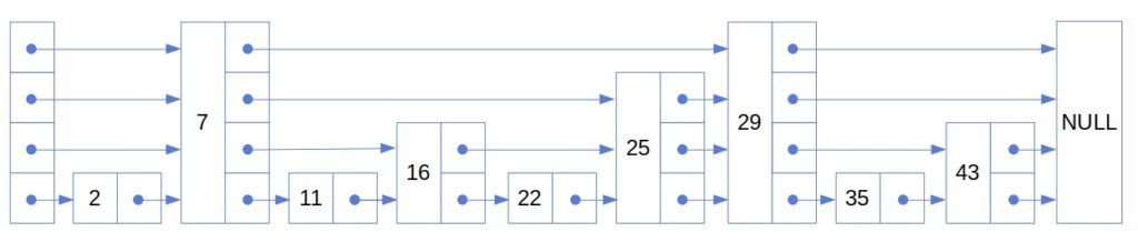
We follow these pointers to find where to place it:

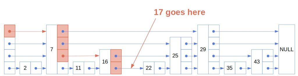
Let’s also say that we chose to set it up as a level-2 node. This is what the list looks like after insertion (the new node and new pointers are in red):

4.3. Complexity

The complexity of insertion, as well as deletion, is dominated by the complexity of the search. To see why, let’s observe that before inserting a new element, we need to locate where to put it. The same goes for deleting a node. We have to find it before deleting it.

5. How to Search Skip Lists

Let’s see how we search a skip list for some value $v$ . It’s similar to inserting $v$ into the list, but we don’t have to update any pointers. We can start at the top level and follow the pointers until we find $\boldsymbol{v}$ or a value greater than $v$ . In the former case, we return the corresponding node. In the latter, we step one level down and repeat the steps. The search ends when we find $\boldsymbol{v}$ or cascade to the bottom-level node greater than $\boldsymbol{v}$ . The node right before it must contain $\boldsymbol{v}$ if the value is in the list. 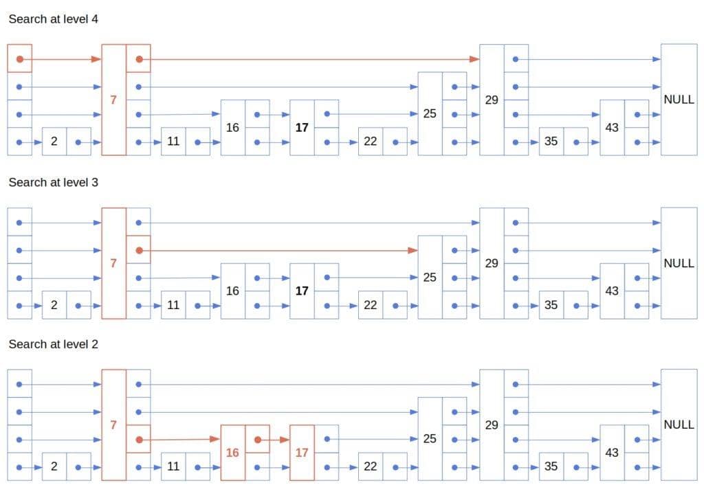Otherwise, we return $failure$ .

5.1. Pseudocode

Here’s the pseudocode of search:

5.2. Example

Here are the steps we make while searching for 17 in the above list:

5.3. The Expected Complexity

We’ll express the expected complexity of the search as the expected length of a search path. It starts in the top-left node (whose level is $\ell = list.maxLevel$ ) and ends in the goal node ( $k \geq 0$ levels below $\ell$ ).

It’s easier to derive the expected length by analyzing the path in reverse. We’ll split it into two parts:

the path to the top-level
the path connecting the top left node (the highest-level head, $list.heads[list.maxLevel]$ ) and the first top node we got to in reverse

Let $L(k)$ be the expected length of the first part. Since skip lists are non-deterministic, we take the expectation over their possible structures. So, from a node $k$ levels below the top, we can either go back one level up with probability $p$ or move left with probability $1-p$ :

$\begin{aligned} L(k) &= 1 + p L(k-1) + (1-p)L(k) \\ p L(k) &= 1 + p L(k-1) \\ L(k) &= \frac{1}{p} + L(k-1) \end{aligned}$

Since $L(0) = 0$ (no need to move to the top level if we’re already at it), we get:

$L(\ell) = \frac{\ell}{p}$

We’ve already solved the second part when we analyzed the number of nodes at different levels. So, we expect the top level to contain $p^{\ell-1}(1-p)n \leq p^{\ell}n$ nodes. Therefore, the total expected complexity of the search is:

(2)

5.4. How to Get the Logarithmic Expected Complexity of Skip Lists

The idea is to choose $\ell$ in such a way that $p^{\ell}n$ becomes a constant $c > 0$ . So, we solve the corresponding equation for $\ell$ :

$\begin{aligned} p^{\ell}n &= c \\ p^{\ell} &= c n^{-1} \\ \ell &= \log_{p}\left(c n^{-1}\right) \\ \ell &= \log_{p}c + \log_{p}n^{-1} \\ \ell &= \log_{p}c + \log_{1/p}n \in O(\log n) \end{aligned}$

So, the first part in Equation (2) becomes $O(\log n)$ , and the second part reduces to $O(1)$ . Therefore, the total expected complexity will be logarithmic if we set $\boldsymbol{\ell}$ to a logarithm of $\boldsymbol{n}$ .

In this analysis, we assumed that $\ell$ was the list’s max level and that we always start the search from the top-level head.

5.5. The Worst-Case Complexity of Skip Lists

In the worst case, the skip list degenerates to a single-linked list, and we’re looking for a value greater than the maximum. So, the worst-case complexity is $\boldsymbol{O(n)}$ because we traverse the whole list.

Even though it’s a pessimistic result, skip lists still pay off. The reasoning is similar to the case of Quicksort with random pivot selection. The theoretically worst possible performance may be poor, but it occurs rarely. In practice, skip lists are very efficient. The logarithmic expected complexity shows it.

6. How to Delete Elements From Skip Lists

Deletion is similar to insertion and search. We first find the node containing the value we want to delete. In the process, we memorize which nodes point to it. If we find the node, we unlink it from its predecessors and point them to the node’s successors at the appropriate levels:

7. Conclusion

In this article, we presented skip lists. We showed three algorithms for skip lists: insertion, search, and deletion. Also, we analyzed the lists as a non-deterministic data structure and showed how to get the logarithmic expected complexity of the search.

Since the complexity of search dominates that of insertion and deletion, the latter two operations can also be made logarithmic. Even though the worst-case complexity is linear, using skip lists still pays off as the worst-case scenario isn’t likely in practice.

Full Archive

About Baeldung

Core Concepts

Operating Systems

Artificial Intelligence

Graph Theory

Latex