

Yes, we're now running our only Summer Sale. All Courses are 30% off until 20th July, 2026:
Create Balanced Binary Search Tree From Sorted List
Last updated: March 18, 2024
Learn through the super-clean Baeldung Pro experience:
>> Membership and Baeldung Pro.
No ads, dark-mode and 6 months free of IntelliJ Idea Ultimate to start with.
1. Overview
In this tutorial, we’ll discuss creating a balanced binary search tree (BST) from a sorted list. Firstly, we’ll explain the meaning of balanced binary search trees.
Then, we’ll discuss the top-down and bottom-up approaches and compare them.
2. Balanced Binary Seach Tree
In the beginning, let’s define the meaning of balanced binary search trees. A balanced binary tree is a tree whose height is  , where
  is the number of nodes inside the tree.
For each node inside the balanced tree, the height of the left subtree mustn’t differ by more than one from the height of the right subtree.
On the other hand, a binary search tree is a binary tree, where the left subtree of each node contains values smaller than the root of the subtree. Similarly, the right subtree contains values larger than the root of the subtree.
Let’s take an example of a balanced binary search tree:
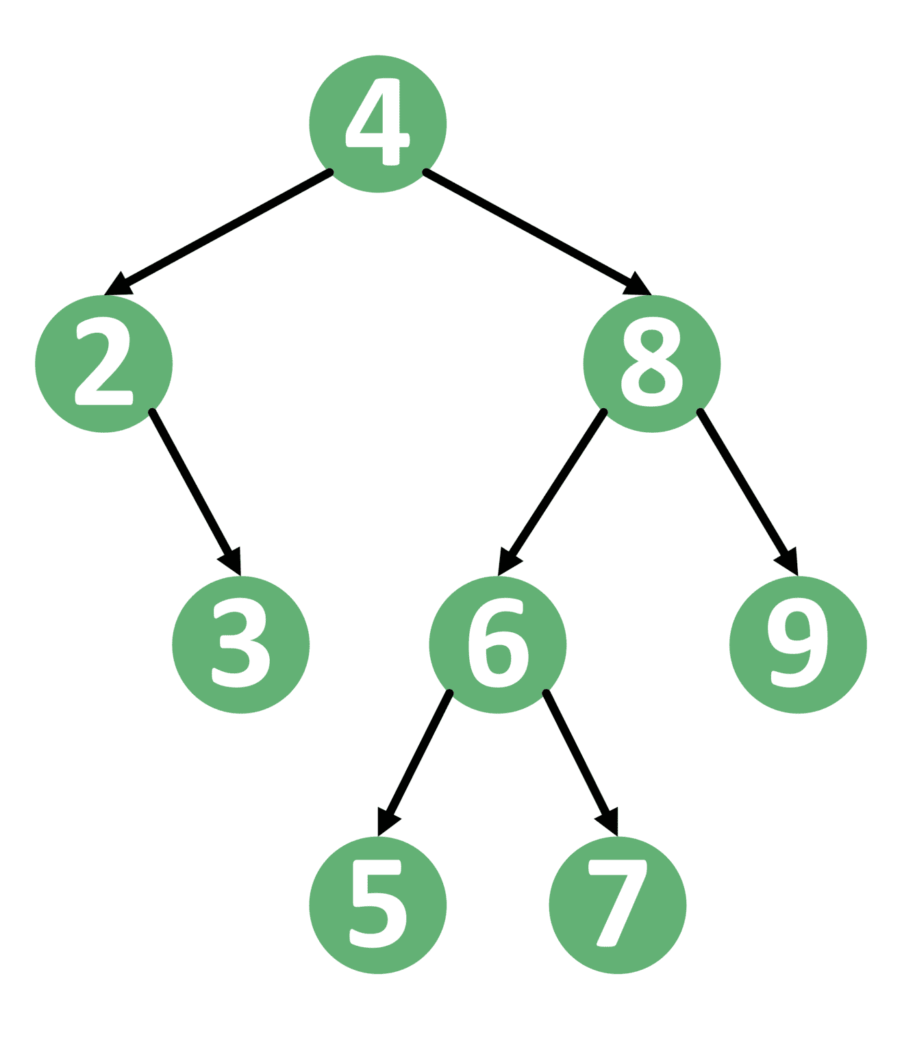
As we can see, the left subtree of the node  contains nodes
  and
and  , which are smaller than . Similarly, the right subtree contains nodes
  , and
, and  , which are larger than .
We can note that this condition holds for all nodes inside the tree. Therefore, this is a binary search tree.
On the other hand, we can note that the left subtree of the node has a height equal to 2. Similarly, the height of the right subtree of the node is 3. Hence, the difference is 1.
We can also note that this condition holds for all nodes inside the tree. Hence, this is a balanced binary search tree.
3. Creating a Balanced BST
When creating a balanced BST we need to keep the height condition in mind. First of all, let’s think about the best node to put as the root.
Since we need the tree to be balanced, we must put the middle value as the root. After that, we can add the values before the middle to the left of the tree. Therefore, all smaller values will be added to the left subtree.
Similarly, we’ll add the values after the middle to the right of the tree, which will cause all larger values to be added to the right subtree.
However, getting the middle element depends on the type of list we have. If the list supports random access, like an array, we can simply get the middle element, put it as the root, then recursively add the left and right subtrees. We call this the top-down approach.
However, if we only have a pointer to the first element in the list, getting the middle element is a little trickier. Therefore, we’ll use the bottom-up approach in this case.
First, we’ll discuss the top-down approach. Then, we’ll move to the bottom-up approach.
4. Top-Down Approach
The top-down approach uses a sorted array to create a balanced BST. Therefore, we can access any index inside the array in constant time.
Let’s have a look at the top-down approach to creating a balanced BST:
algorithm TopDownBST(A, L, R):
    // INPUT
    //   A = The sorted array
    //   L = The left side of the current range
    //   R = The right side of the current range
    // OUTPUT
    //   The root of the balanced BST

    if L > R:
        return null

    mid <- (L + R) / 2

    root.value <- A[mid]
    root.left <- TopDownBST(A, L, mid - 1)
    root.right <- TopDownBST(A, mid + 1, R)

    return root
The initial call for this function passes the array  , the value of
  is zero and
  is
is  , where is the size of the array.
In the beginning, we check to see if we reached an empty range. In this case, we simply return  , indicating an empty object.
Next, we get the middle index and initiate the root node with ![A[mid]](/wp-content/ql-cache/quicklatex.com-00342b288d9746ff20b057356c46f10b_l3.svg "Rendered by QuickLaTeX.com") . After that, we make two recursive calls. The first call is for the range
. After that, we make two recursive calls. The first call is for the range ![[L, mid-1]](/wp-content/ql-cache/quicklatex.com-1d4fff429c290a61946f52fd85d77b30_l3.svg "Rendered by QuickLaTeX.com") , which represents the elements before the index
, which represents the elements before the index  . On the other hand, the second call is for the range
 ![[mid+1, R]](/wp-content/ql-cache/quicklatex.com-b271f25e0c563ad38ada9892840eec6f_l3.svg "Rendered by QuickLaTeX.com") , which corresponds to the elements after the index .
, which corresponds to the elements after the index .
The first call returns the root of the left subtree. Therefore, we assign its value to the left pointer of the root node. Similarly, the second call returns the root of the right subtree. Hence, we assign its value to the right pointer of the root node.
The complexity of the top-down approach is  , where is the number of elements inside the array.
5. Bottom-Up Approach
The bottom-up approach uses a linked list to build a balanced BST. As a result, we’ll have a pointer to the head of the list and we can only move this pointer forward in constant time.
Take a look at the bottom-up approach to creating a balanced BST:
algorithm BottomUpBST(head, L, R):
    // INPUT
    //   head = Pointer to the first element in the linked list
    //   L = The left side of the current range
    //   R = The right side of the current range
    // OUTPUT
    //   The root of the balanced BST

    if L > R:
        return null

    mid <- (L + R) / 2

    // Build left subtree
    root.left <- BottomUpBST(head, L, mid - 1)

    // Assign root value
    root.value <- head.data

    // Move to the next element in the list
    head <- head.next

    // Build right subtree
    root.right <- BottomUpBST(head, mid + 1, R)

    return root
The initial call for this function is similar to the top-down approach. We’ll pass a pointer the beginning of the list  , the value of is zero and is , where is the number of elements.
First, we check whether we have reached an empty range. If so, we return indicating an empty tree.
Then, We build the left subtree recursively. Next, since the left subtree is completely built, it means the pointer is now pointing to the element with index . Therefore, we store its value inside the root.
After that, we move the pointer one step forward because when the recursive call for the left subtree finished, we assumed that the pointer was on the mid element. Hence, we need to move the pointer forward so that the next recursive call can use it from there.
Finally, we perform a recursive call to build the right subtree and then return the root node.
The reason for calling this approach bottom-up is that we keep going into recursive calls until we reach the leftmost node. We create this node and then move to other recursive calls to build their nodes as well.
The complexity of the top-down approach is , where is the number of elements inside the linked list.
6. Comparison
| Top-Down | Bottom-Up | |
|---|---|---|
| Main Idea | Create the middle node. Then, recursively create the left and right subtrees | Keep going recursively to the leftmost node. reate it, and move to the next node |
| Data Structure | Sorted array | Sorted linked list |
| Complexity | O(n) | O(n) |
Usually, the top-down approach is considered easier to understand and implement, because it’s straight forward. On the other hand, the bottom-up approach needs a little more understanding of the recursive calls, and how exactly is the tree built from the leftmost to the rightmost node.
Both approaches have the same time complexity. However, each approach is based on a different data structure.
If the data is inside a sorted array, then using the top-down approach is usually easier than the bottom-up approach. On the other hand, if the data is inside a sorted linked list, then we need to use the bottom-up approach.
7. Conclusion
In this tutorial, we presented two approaches to building a balanced binary search tree from a sorted list.
Firstly, we explained the general concept of balanced binary search trees. Secondly, we presented the top-down approach and the bottom-up approach.
In the end, we compared both approaches and showed when to use each one.