Scale-Invariant Feature Transform | Baeldung on Computer Science

1. Overview

In this tutorial, we’ll talk about the Scale-Invariant Feature Transform (SIFT). First, we’ll make an introduction to the algorithm and its applications and then we’ll discuss its main parts in detail.

2. Introduction

In computer vision, a necessary step in many classification and regression tasks is to detect interesting points (also called keypoint detection). Then, for each point, it is also useful to provide a feature description that is invariant in scaling, rotation, and illumination changes. These properties are necessary to ensure that the points are detectable even under these transformations in an image.

After computing a descriptor for each point of interest, we can use them for classification tasks like detecting objects in an image. Also, they are useful in image matching where our goal is to match points between different views of a 3-D scene.

A well-known and very robust algorithm for detecting interesting points and computing feature descriptions is SIFT which stands for Scale-Invariant Feature Transform.

3. Main Steps

Now, let’s discuss the algorithm behind SIFT step-by-step. We’ll assume that we have an input image $I$ with width $w$ and height $h$ .

3.1. Scale-Space

The first step is to compute the scale-space of the image which is the result of the convolution of a Gaussian kernel $\mathbf{G}$ at different scales with the image $\mathbf{I}$ . But, why do we need this?

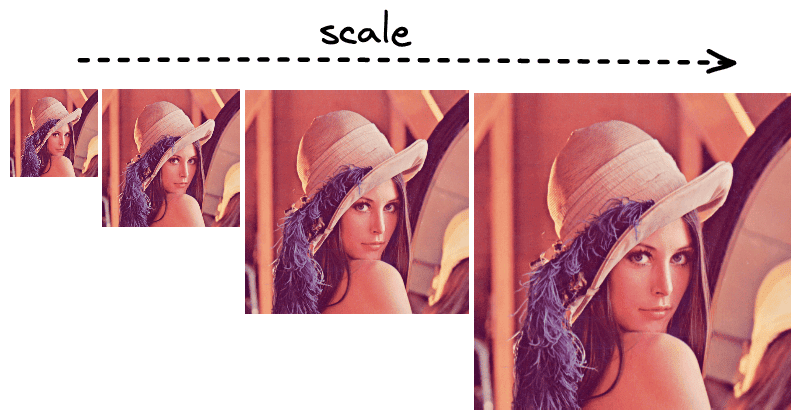
Objects in the real world are discriminative at certain scales. For example, in the below figure the eyes of the woman are more discriminative in the right image where the scale is large while the hat (a large object) is more discriminative in smaller scales (left image):

So, we need to represent an image in multiple scales to infer interesting points across many scales. To achieve this, we use the Gaussian kernel that is defined as:

$G(x, y, \sigma) = \frac{1}{2 \pi \sigma^2} \e^\frac{-(x^2 + y^2)}{2\sigma^2}$

where $x$ , $y$ are the coordinates of each pixel and $\sigma$ is the parameter related to the scale.

To represent an image $\mathbf{I}$ in multiple scales, we compute the convolution of the image with the kernel at each scale. The equation is defined as:

$L(x, y, \sigma) = G(x, y, \sigma) \ast I(x, y)$

3.2. Find Keypoints using DoG

The next step is to find the interesting points using the Difference of Gaussians (DoG). Specifically, we take the different versions of the image according to the scale and compute their differences.

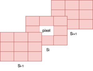
Then, we compare the value of each pixel with its 8 neighbors in the same scale as well as the 9 pixels in the next and in the previous scale. In case its value is smaller or larger than all of these values it is considered a possible interest point.

In the diagram below, we can see in orange the pixels that we have to compare with a specific point:

However, the points that satisfy the above condition are many and we want to keep only the most discriminative. So, we compare the intensity of each point with a predefined threshold and keep only the ones that are above the threshold.

3.3. Compute Orientation

Now that we have detected some interesting points at certain scales, we also want to compute their orientation. So, we define an orientation histogram of 36 bins that covers $360^{\circ}$ in total. Each bin $i$ contains the degrees in the range $[i*10, (i+1)*10)$ .

For example, if the gradient direction of a pixel is $32^{\circ}$ and the gradient amplitude is 10, then we add the value of 10 in the 4th bin.

In the below image, we can see how a sample histogram looks:

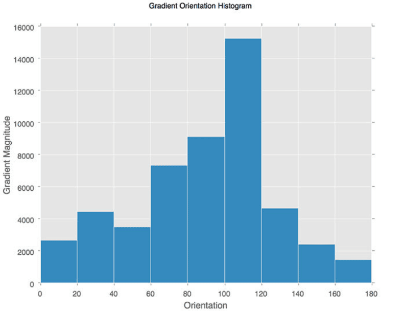
We compute a histogram like the above for each interesting point. The orientation of the point is the angle with the maximum value in the histogram.

3.4. Compute Descriptors

At this stage, we have some interesting points along with their location, their scale, and their orientation. The final step is to compute a descriptor for the region around each detected point.

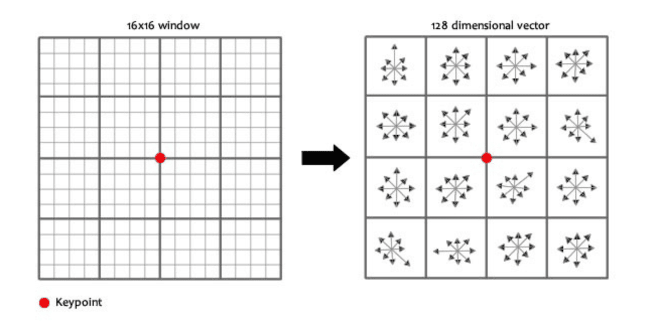
First, we take a patch of size $16 \times 16$ around each point and divide it into 16 sub-blocks of $4 \times 4$ size. For each sub-block, we compute an 8-bin orientation histogram as in the previous step. So, we end up with $8 \times 4 \times 4 = 128$ values. These 128 values correspond to the feature vector of the point.

Below, we can see the computation of the feature vector for a certain point:

Finally, we end up with one feature vector of size 128 for each interesting point. These vectors can then be used for any computer vision task we want since they contain all the useful discriminative information we might want.

6. Conclusion

In this tutorial, we presented the Scale-Invariant Feature Transform (SIFT). We first made a brief introduction to the algorithm and then we discussed each step of the method independently.

Full Archive

About Baeldung

Core Concepts

Operating Systems

Artificial Intelligence

Graph Theory

Latex