

Yes, we're now running our only Summer Sale. All Courses are 30% off until 20th July, 2026:
Mean Average Precision in Object Detection
Last updated: February 12, 2025
Learn through the super-clean Baeldung Pro experience:
>> Membership and Baeldung Pro.
No ads, dark-mode and 6 months free of IntelliJ Idea Ultimate to start with.
1. Overview
In this tutorial, we’ll talk about the mean average precision (mAP) metric that is used to evaluate an object detection model. First, we’ll make a brief introduction to the task of object detection. Then, we’ll present the overlap criterion and the precision and recall metrics. Finally, we’ll talk about how to calculate the final mAP metric.
2. Object Detection
The goal of object detection is to locate and identify the depicted objects in an image. It is one of the most important tasks in computer vision, with applications ranging from autonomous driving and security to retail and healthcare. Generally, the task of object detection involves two steps:
- Object localization: we want to predict the location of one or more objects in an image and draw a bounding box around each of them
- Image classification: we want to predict the class of each object in the image
So, an object detection system takes as input an image with one or more objects and outputs one or more bounding boxes along with a class label for each bounding box. The task of object detection is also referred to as object recognition.
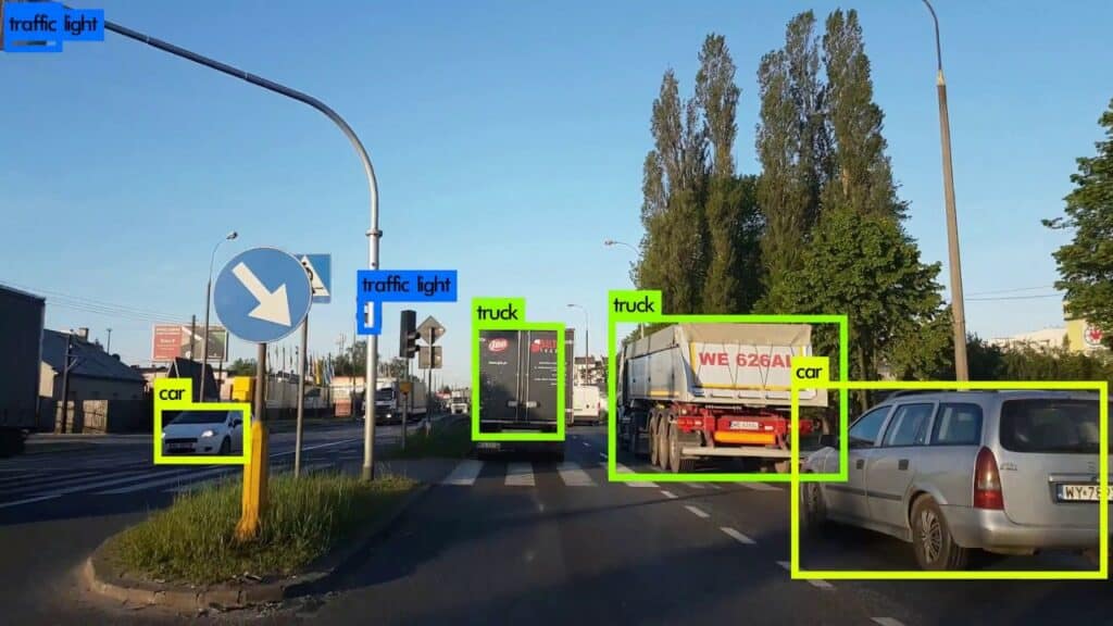
In the image below, we can see a possible output of an object detection system if the input is an image that depicts a road. We observe that the model has successfully localized six objects by drawing a rectangle around them and has correctly classified them in their respective classes (traffic light, truck, and car):
Over the past years, many deep learning models have been proposed for the task of object detection achieving exciting performance like R-CNN and YOLO. To evaluate their performance, we need to define a proper metric.
As an input to the metric, we have the predicted bounding boxes along with the predicted classes. How to compare these values with the actual bounding boxes and classes in a consistent and quantitative way? The most popular metric to evaluate an object detector is mean Average Precision (mAP).
3. Overlap Criterion
The first step in computing the mAP is to find the degree of overlap between the ground truth and the predicted bounding boxes. The most common overlap criterion is the Intersection over Union (IoU) that takes the predicted bounding box A and the ground truth bounding box B and calculates:

where  denotes their intersection and
  denotes their union. In the diagram below, the definition of IoU is shown diagrammatically:
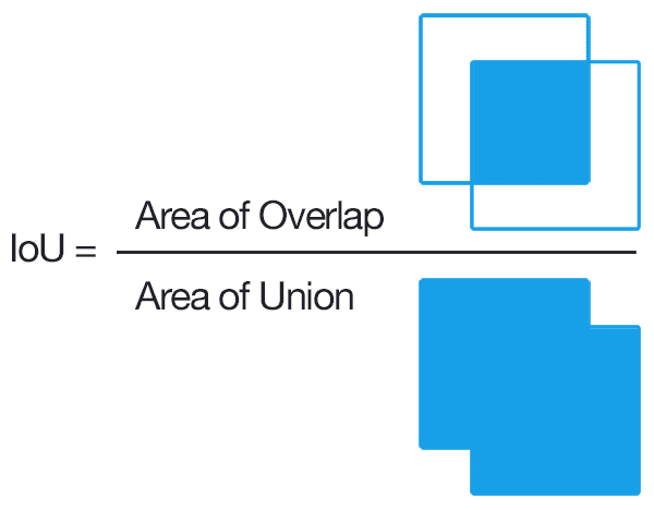
We observe that the value of IoU lies between 0 and 1, where 0 means no overlap at all and 1 means perfect overlap between the predicted and the ground truth bounding box. To check if the detection is correct, we need to define a threshold that is able to account for small inaccuracies in the prediction that don’t affect the final output. Usually, the threshold is equal to 50%, and the detection is considered successful when  .
.
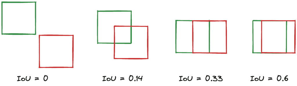
In the image below, we can see some examples of computing the IoU in two bounding boxes. The detection succeeds only in the last case:
4. Precision and Recall
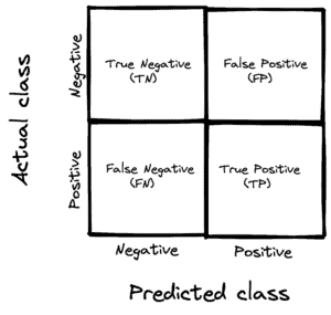
Now that we have a way to decide if a detection succeeded, we can convert the localization problem to a binary classification problem where the positive class means that the object was detected. We know that in every binary classification problem, a prediction can be a true-positive, false-positive, true-negative, or false-negative based on the table below:
Also, we use the terms precision and recall to evaluate the performance of the classification:
- Recall measures the ability of the model to detect all ground truths:

- Precision is how successful is the model in identifying only relevant objects:

Of course, we want a model to have high precision and high recall. To take into account both metrics, we use the Precision-Recall Curve, which is a plot of the precision (y-axis) and the recall (x-axis) for different probability thresholds.
We compute Average Precision (AP) by averaging the precision values on the precision-recall curve where the recall is in the range [0, 0.1, …, 1]:

where ![i \in [0, 0.1, ..., 1]](/wp-content/ql-cache/quicklatex.com-cc80e9ecf057dffb4129c2dcf69f4b7f_l3.svg "Rendered by QuickLaTeX.com") and
and  denotes the value of the precision when the recall is equal to
  .
.
5. Mean Average Precision (mAP)
Until now, we haven’t talked about the classification part of the detection. We want not only to compute the bounding box of each object but also to predict its class.
So, we compute the AP for each class individually and end up with  values of AP where is the number of classes. Our final metric is mAP which is equal to the average of AP values for all classes:

where  is the value of AP for class .
6. Conclusion
In this tutorial, we presented the mAP metric for object detection. First, we talked about the task of object detection and defined the overlap criterion and the precision and recall metrics. Then, we discussed how to calculate the mAP metric.