

Learn through the super-clean Baeldung Pro experience:
>> Membership and Baeldung Pro.
No ads, dark-mode and 6 months free of IntelliJ Idea Ultimate to start with.
Learn through the super-clean Baeldung Pro experience:
>> Membership and Baeldung Pro.
No ads, dark-mode and 6 months free of IntelliJ Idea Ultimate to start with.
In this tutorial, we’ll present some algorithms for image comparison. First, we’ll make an overview of the problem and then we’ll introduce three algorithms from the simplest to the most complex.
In image comparison, we have two input images  and
and  and our goal is to measure their similarity
  . First, we have to realize that the concept of similarity is not strictly defined and can be interpreted in many ways. Specifically, two images
  and
and  can be considered similar if:
Below, we can see different interpretations of image similarity. The left image is a rotated version of the original image with a distinct contrast, while the right image depicts the same dog but in a different background:
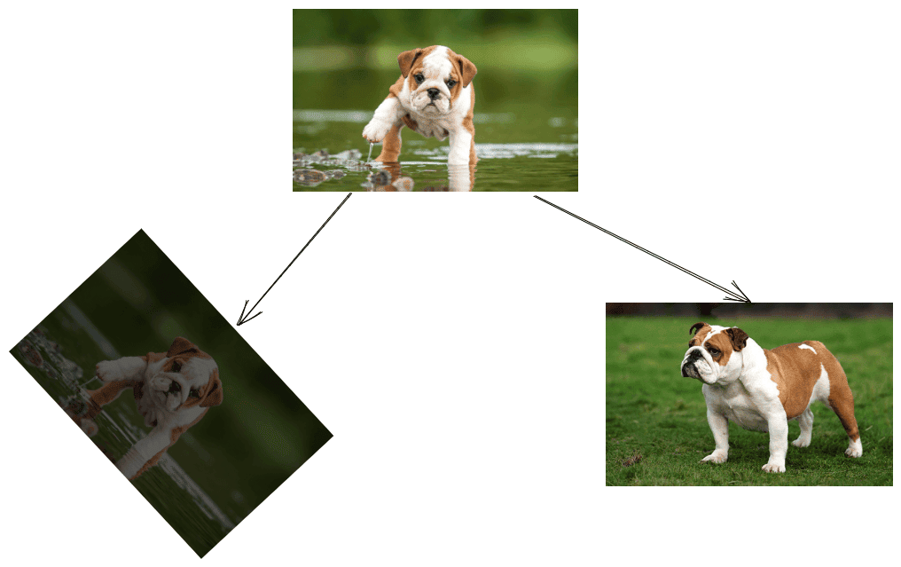
We realize that it is much easier to implement an image comparison system for the left case since the dog’s pose and background surface remain the same.
In this tutorial, we’ll present algorithms that compare images based on the content starting from the simplest to the most complex.
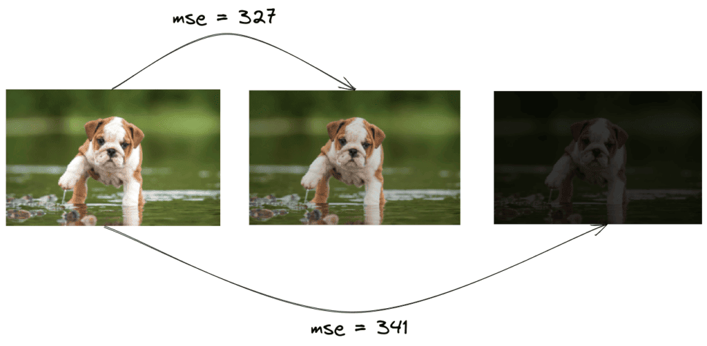
A naive approach would be to use a metric that takes as input the raw pixels of the images and outputs their similarity. We can use the classical Mean Squared Error in this case to compute the mean value of the square of the differences between the pixels of the two images:

We can assume that the lower the value of MSE, the higher the similarity. Despite its speed and simplicity, this method comes with many problems. Large Euclidean distance between pixel intensities does not necessarily mean that the image’s content is different.
As we can see below, if we just change the contrast of the image, the final MSE value will increase a lot, although we did not change the content:
Pixel-based methods like MSE are not effective when the input images are taken under different angles or lighting conditions. To deal with these cases, image matching is the appropriate method.
The first step in image matching is to detect some points in the input images that contain rich visual information. These points usually correspond to the edges and the corners of the objects in the image. The most well-known key point detectors are Harris corner detector, SIFT and SURF.
Below, we can see an example of applying a key point detector to the previous images. The detected key points are shown in purple:
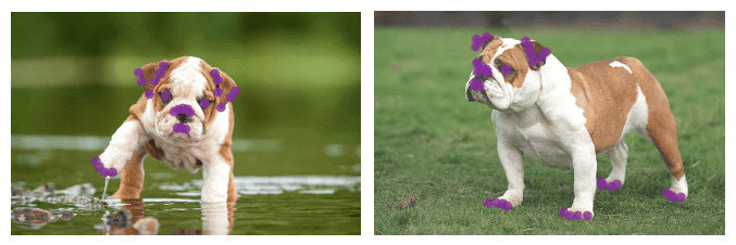
We observe that the key points are located in the region of the eyes, the ears, the mouth and the legs of the dog.
Our next step is to compute a local descriptor for each detected key point. A local descriptor is defined by a 1-dimensional vector that describes the visual appearance of the point. As a result, points from the same parts of the object will have similar vectors. The aforementioned SIFT and SURF methods are able to compute the local descriptors after detecting the key points.
The final step is to match the descriptors of the two images. To do this, we iteratively compare the descriptors of the images to discover pairs of descriptors that are similar. If the amount of similar descriptors is above a certain threshold, then it means that the two images depict the same object and are considered similar.
Below, we have matched the points located in the left ear and the front right leg of the dog in the two images:
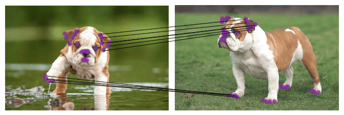
Image matching using keypoint detectors and local descriptors is a successful image comparison method. One possible downside is the running time of the final step of the algorithm that is  where
where  is the number of the detected key points. However, there are other algorithms that perform the matching step between the key points faster using quadtrees or binary space partitioning.
Despite its intuitiveness, image matching cannot generalize well in real-world images. Its performance depends on the quality of the key point detector and the local feature descriptor. Now, we’ll move on to the best image comparison algorithm nowadays that uses Siamese Networks.
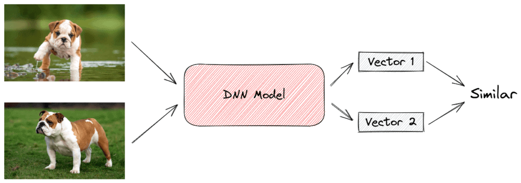
A Siamese Network is a neural network that consists of two identical subnetworks meaning that they contain exactly the same parameters and weights. Each subnetwork can be any neural network designed for images like a Convolutional Neural Network. The network’s input is a pair of images that are either similar (positive example) or not similar (negative example).
During training, we pass the images through the subnetworks, and we get as output two feature vectors, one for each image. If the input pairs are similar, we want these two vectors to be as close as possible and vice versa. To achieve this, we use the contrastive loss function that takes a pair of vectors  and minimizes their euclidean distance when they come from similar images while maximizing the distance otherwise:

where  if the images are similar and
  otherwise. Also,
  is a hyperparameter, defining the lower bound distance between images that are not similar.
In the below images, we can see the siamese architecture in the case of positive and negative examples:
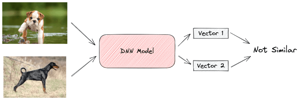
After training, the network has successfully learned to compare any pair of images using the euclidean distance of their output vectors (small distance corresponds to high similarity).
Using Siamese networks, we are able to compare images with high precision even in the most extreme conditions (low-quality images, blurring, occlusions, etc.). The only downside is that this is a learning-based method requiring a labeled image dataset for training.
In this tutorial, we discussed three algorithms for image comparison. First, we made a brief introduction to the problem. Then, we presented the algorithms along with illustrative examples.