Salp Swarm Algorithm | Baeldung on Computer Science

1. Introduction

In this tutorial, we’ll go through the details of a relatively new nature-inspired meta-heuristic optimization technique. This is inspired by the swarming behavior of sea salps that are often found in deep oceans.

It’s an active area of research but has already proven helpful in specific optimization problems.

2. What Is Salp Swarm?

Salp is a barrel-shaped planktic tunicate that belongs to the family of Salpidae. It exhibits one of the most efficient examples of jet propulsion in the animal kingdom. This is when it moves by contracting, thereby pumping water through its gelatinous body.

One of the interesting behaviors of salps is when it forms a stringy colony by aligning next to each other:

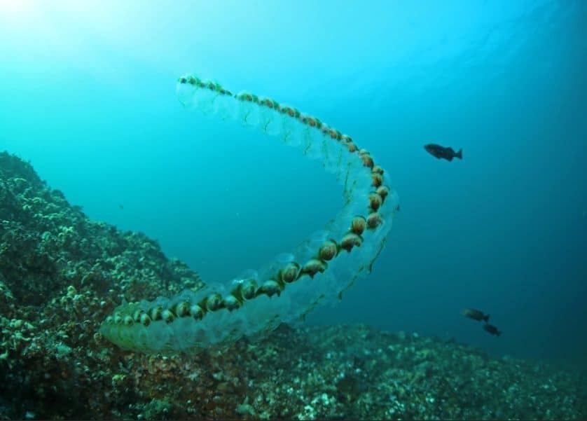
From a biological perspective, it’s not clear about the reason for this swarming behavior of salps. But researchers have indicated that this may be done for better locomotion and foraging. We refer to the swarm of salps as a salp chain, and at times, they can be quite enormous!

3. Why Is This of Interest to Us?

Salps are fascinating creatures, and much research is still underway to understand them better in their natural habitat. But, for the interest of optimization problems, their swarming behavior is most peculiar to us. The key is to mimic this behavior in solving complex optimization problems. We’ll see why this is of interest to us.

Swarm Intelligence is the collective behavior of decentralized, self-organized systems. These systems can be natural or artificial but typically consists of simple agents interacting locally with one another and their environment. While the agents follow simple rules, their interaction leads to the emergence of intelligent global behavior.

The optimization problems in real life are often very complex in nature. The search space they generate is often quite tricky for mathematical programming to find a globally optimal solution in limited time and resources. This is where metaheuristics can promise to find suitable solutions in less computational effort. Although, they do not guarantee to find the globally optimal solution.

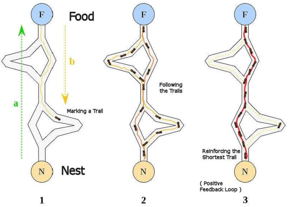
The swarming behavior of natural agents like ants, grasshoppers, whales, bees, glowworms has been studied for several years to develop metaheuristics for solving such complex optimization problems. They all exhibit solving complex problems as a whole, which isn’t possible for them individually. For instance, ants are cooperatively able to find food sources even far from their nest:

Interestingly, while a particular metaheuristic can solve a specific set of optimization problems, it might not perform that well on others. This is what precisely keeps the research in this field thriving. We seek to understand if we can learn and model the behavior of salp swarm to solve specific optimization problems more efficiently?

4. Mathematical Modelling

While the concept itself is quite appealing, it would not take us anywhere unless we can mathematically model the swarming behavior of salps. One of the earliest attempts to do so has been presented by S. Mirjalili et. al. in their research paper published a few years back. To achieve this, they have proposed to divide the salp population in a swarm into a leader and followers:

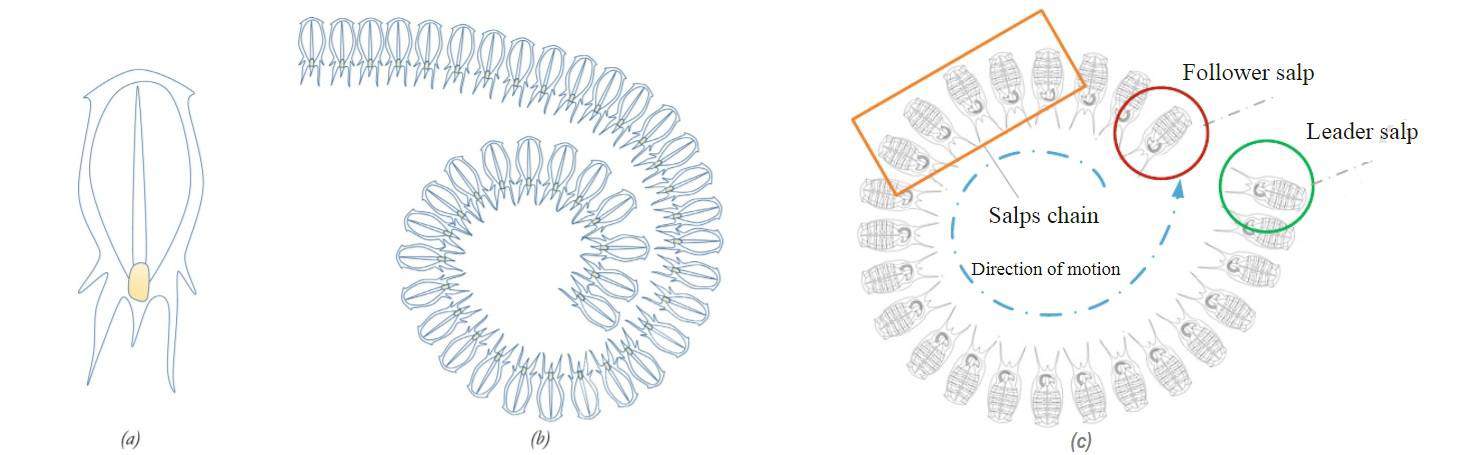
As we can see in the above schematic, single salps (a) come together to form a salp chain (b). For the purpose of mathematical modeling, we designate the first salp in the direction of motion of the salp chain as the leader salp and the rest of the salps as follower salps (c).

We begin by defining the position of salps in an $n$ -dimensional search space where $n$ is the number of variables in a given problem. We can store the position of all salps in a two-dimensional matrix called $x$ and designate the food source as $F$ in the search space.

Now, we can update the postion of the leader salp using this equation:

$x_{j}^{1} = \left\{\begin{matrix} F_{j} + c_{1}((ub_{j} - lb_{j})c_{2} + lb_{j}) \hspace{1cm} c_{3} \geqslant 0 \\ F_{j} - c_{1}((ub_{j} - lb_{j})c_{2} + lb_{j}) \hspace{1cm} c_{3} < 0 \end{matrix}\right.$

Here, $x_{j}^{1}$ denotes the position of the leader salp in the $j$ th dimension, and $F_{j}$ denotes the position of the food source in the $j$ th dimension. Further, $ub_{j}$ and $lb_{j}$ represent the upper and lower bounds of the $j$ th dimension, respectively.

Also, $c_{1}$ , $c_{2}$ , $c_{3}$ are random variables. As we can see, out of these coefficients, $c_{1}$ is most important as it helps in balancing between exploration and exploitation. We can update this coefficient as:

$c_{1} = 2e^{-(\frac{4l}{L})^{2}}$

The coefficients $c_{2}$ and $c_{3}$ are random numbers uniformly generated in the interval $[0,1]$ . They dictate the next position in the $j$ th dimension and the step size.

Interestingly, the leader salp only updates its position with respect to the food source. The follower salps update their position with respect to each other, and hence the leader salp ultimately.

We can use the equation from Newton’s laws of motion to update the position of the follower salps. With certain modifications apt to the domain of optimization problems, we arrive at this equation:

$x_{j}^{i} = \frac{1}{2}(x_{j}^{i} + x_{j}^{i-1}) \hspace{1cm} i \geqslant 2$

Here, $x_{j}^{i}$ denotes the position of the $i$ th follower salp in the $j$ th dimension.

With these equations, finally, we can reasonably simulate the behavior of the salp swarm mathematically. We can use this mathematical model to develop algorithms for solving optimization problems.

5. Salp Swarm Algorithms

Now that we’ve got a mathematical model for the salp swarm, it’s time to use it to create an algorithm to solve some of the optimization problems. Of course, the model can not be used as is to solve these problems. We need to adapt parts of it to suit the problem at hand. An optimization problem can be either single objective or multi-objective, and the algorithm will have to be specific to each.

5.1. Single Objective Problems

A single-objective optimization problem, as the name suggests, has only one objective to chase. The objective is either to maximize or minimize. These can further have a set of equality or inequality constraints. We can mathematically formulate these problems like:

$Minimize: F(\vec{x}) = {f_{1}(\vec{x})}$

$Subject to: g_{i}(\vec{x}) \geqslant 0, i = 1,2,3,...,m$

$h_{i}(\vec{x}) = 0, i = 1,2,3,...,p$

$lb_{i} \leqslant \vec{x} \leqslant ub_{i}, i = 1,2,3,...,n$

This formulation is for minimizing the objective function with $n$ number of varaibles, subject to $m$ inequality constraints and $p$ equality constraints. Further the $i$ th variable has $lb_{i}$ and $ub_{i}$ as its lower and upper bound respectively.

To solve this problem using the mathematical model of the salp swarm, we begin by replacing the food source with the optimal global solution. Since we do not know this in advance, we can assume the best solution obtained so far as the global optimum and assume the salp chain to chase this.

Hence, we get the pseudo-code of the algorithm for solving a single-objective optimization problem with the salp swarm model:

The author of the original paper refers to this algorithm as the Single-objective Salp Swarm Algorithm (SSA). We begin by initiating multiple salps with random positions. Then we calculate the fitness of each salp to find the salp with the best fitness. This is followed by coefficient updates and updates to the position of the leader and the follower salps. This becomes our current global optimum.

Now, because the leader salp updates its position only with respect to the current optimal solution, it allows for exploration and exploitation of space around it. Moreover, the gradual movement of follower salps prevents potential stagnation in locally optimal solutions. The salp chain will likely move towards the actual global optimum throughout multiple iterations.

5.2. Multi-Objective Problems

As we can guess, multi-objective problems have multiple objectives to deal with and all the objectives should be optimized simultaneously. Their mathematical formulation looks quite similar to the one for single objecvtive problems, only with multiple objectives:

$Minimize: F(\vec{x}) = {f_{1}(\vec{x}), f_{2}(\vec{x}), f_{3}(\vec{x}), ..., f_{o}(\vec{x})}$

$Subject to: g_{i}(\vec{x}) \geqslant 0, i = 1,2,3,...,m$

$h_{i}(\vec{x}) = 0, i = 1,2,3,...,p$

$lb_{i} \leqslant \vec{x} \leqslant ub_{i}, i = 1,2,3,...,n$

Here, the formulation has $o$ objective functions to minimize the rest of the description, as seen earlier.

Now, with a single objective, it’s quite clear to compare candidate solutions using the relational operators. However, with multiple objectives, this gets quite complicated. For this, we refer to a concept called Pareto optimal dominance. We can define this mathematically as:

$\vec{x} \prec \vec{y} \leftrightarrow \forall{i} \in \left\{ 1,2,3, ...,k \right\}, \left [ f_{i}(\vec{x}) \leqslant f_{i}(\vec{y}) \right ] \wedge \exists{i} \in \left\{ 1,2,3, ...,o\right\}, \left [ f_{i}(\vec{x}) < f_{i}(\vec{y}) \right ]$

This may look intimidating, but it simply states that a solution, represented by $\vec{x}$ is better than another, represented by $\vec{y}$ , if and only if it has equal and at least one better value in the objectives. In such a case, a solution is said to dominate the other. Otherwise, the solutions are said to be Pareto optimal or non-dominated solutions.

There is a set of Pareto optimal solutions in multi-objective optimization problems that we call a Pareto optimal set. The projection of the Pareto optimal set in the objective space is called Pareto optimal front.

The first step to adopt the mathematical model for the salp swarm for solving this kind of problem would be to replace the one optimal solution with a repository of non-dominated solutions with a maximum limit. The second step would be to select the food source from a set of non-dominated solutions with the least crowded neighborhood.

So, we can update the pseudo-code for the algorithm to solve multi-objective problems with the salp swarm model as:

The author of the original paper refers to this algorithm as the Multi-objective Salp Swarm Algorithm (MSSA). The algorithm is mainly similar to what we discussed earlier for SSA, with a few changes to accommodate that we’re dealing with multiple objectives now! The most significant difference is that we’ve got a repository of non-dominated solutions to maintain now.

There are, of course, more complexities to this algorithm that we’ve not covered. For instance, how to deal with the situation where the repository is full, and we’ve got a salp that is non-dominated compared to the repository residents. The algorithm suggests swapping it with a repository resident. But how to pick which repository resident to delete?

We can assign a rank to each repository resident based on the number of neighboring solutions and then choose a roulette wheel to choose one of them. This approach helps improve the distribution of the repository resident over the course of iterations. While inheriting all the merits of SSA, this algorithm also leads the search towards the less crowded regions of the Pareto optimal front.

6. Practical Applications

Algorithms based on the salp swarm are an active area of research, and we’re finding it helpful in new ways as it’s progressing. As we’ve seen earlier, a metaheuristic algorithm typically performs better than others only on a particular set of optimization problems. We can not expect such an algorithm to outperform others in the general class of problems.

In the original paper, the authors presented a set of qualitative metrics and collected quantitative results to compare SSA with similar algorithms. They have also compared the MSSA algorithm with similar algorithms in the literature. A detailed analysis of these comparisons is beyond the scope of this article.

However, the authors have also presented the performance of SSA and MSSA in a certain class of real-world problems. These include classical optimization problems like three bar truss design problem, welded beam design problem, I-beam design problem, cantilever beam design problem, tension/compression spring design problem.

This also includes employing SSA to solve the two-dimension airfoil design problem and MSSA for the marine propeller design problem. It’s evident from the results that the SSA and MSSA can find optimal shapes for these problems. Of course, further research in this area will prove the efficiency of these algorithms and find more practical applications like optimization of Extreme Machine Learning (ELM)!

7. Conclusion

In this tutorial, we understood the details of salp swarm and how they can interest us in optimization problems. Further, we went through the mathematical modeling of the salp swarm and adapted it to create metaheuristic algorithms. This covered algorithms for solving single-objective and multi-objective problems.

Full Archive

About Baeldung

Core Concepts

Operating Systems

Artificial Intelligence

Graph Theory

Latex