Grasshopper Optimization Algorithm | Baeldung on Computer Science

1. Overview

There are various optimization algorithms in computer science, and the Grasshopper Optimization Algorithm (GOA) is one of them. In this tutorial, we’ll take a look at what this algorithm means and what it does.

Then, we’ll go through the steps of the GOA algorithm. In addition to a numerical example demonstrating the solution of an optimization issue using GOA, we’ll discuss its benefits and drawbacks.

2. What Is the Grasshopper Optimization Algorithm?

GOA is a meta-heuristics algorithm and a population-based algorithm. As implied by the name, this algorithm was proposed for solving numerical optimization issues by Saremi and Mirjalili, 2017. It’s a recent swarm intelligence algorithm. The inspiration for GOA comes, in particular, from the behavior and the interaction of grasshopper swarms in nature.

3. Who Are the Grasshoppers?

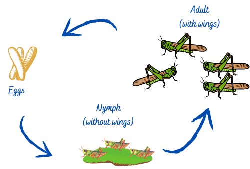
Grasshoppers are harmful and destructive insects because of the extensive damage they cause to crops. Let’s take a look at the life cycle of grasshoppers, which has three phases:

Egg: The initial phase involves egg-laying in a pod on the ground near a feeding plant in the summer. This stage lasts a few weeks before going into diapause in the winter. Then, as soon as the ground temperature increases, the egg resumes its development and hatch to become first instar Nymph
Nymph: They mature in stages, with each instar becoming more and more like an adult. The first instar nymph doesn’t have wings. However, the nymph has to go through six stages to become an adult, and the wing-buds grow in size at each stage. Therefore, they move slowly and eat each vegetation on their path
Adulthood: The wings are expanded and fully functional after the final instar stage. So, they form a swarm in the air and move fast to a large-scale region

In short, the Grasshopper life cycle may resemble the image below:

Let’s now investigate the main characteristic of the grasshopper swarm:

The swarm moves slowly using small steps in the nymph phase because they don’t have wings
The grasshopper swarm can make sudden jumps and long-range moves in the phase of adulthood because they have wings. This phase represents the main idea behind the GOA algorithm
The swarm searches for food by splitting the process into two stages: exploration and exploitation. The graph below presents these phases:

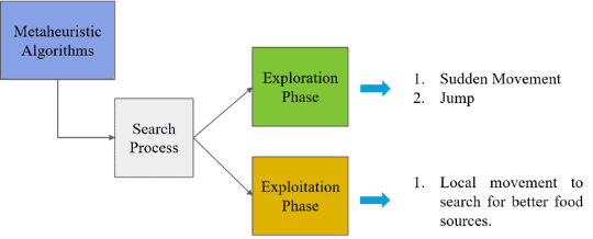
In the exploration phase, the swarm search for food sources. Thus, in this stage, we update all the value positions of the grasshopper and compute the fitness value. In the exploration phase, we find the best solution among all solutions (search for better food sources).

4. Mathematical Model of the Grasshopper Optimization Algorithm

The GOA algorithm mimics the social behavior and hunting method of grasshoppers in nature. It’s a population-based algorithm, with each grasshopper representing a solution in the population. So, how do we determine the position of each solution in the swarm?

It’s simple, we only need to calculate three forces: the social interaction between the solution and the other grasshoppers, the wind advection, and the gravity force on the solution. Let’s now have a look at the mathematical model used to calculate the position ${X_i}$ of each solution:

(1) $\begin{equation*} {X_i} = {S_i} + {G_i} + {A_i} \end{equation*}$

where ${S_i}$ represents the social interaction between the solution and the other grasshoppers, ${G_i}$ represents the gravity force on the solution, and ${A_i}$ represents the wind advection. The equation below represents the position of each solution after adding random behavior to it:

(2) $\begin{equation*} {X_i} = {r_1} {S_i} + {r_2} {G_i} + {r_3} {A_i} \end{equation*}$

where ${r_1}, {r_2},$ and ${r_3}$ are random numbers in [0, 1]. Let’s now have a look at the model of each force used in Equation 1.

Let’s firstly start with the force of social interaction ${S_i}$ . The equation below represents the social interaction between the solution and the other grasshoppers:

(3) $\begin{equation*} {S_i} = \sum_{j=1}^{N} s({d_{ij}}) \hat{d_{ij}} \text{ , where } {i} \neq {j} \end{equation*}$

(4) $\begin{equation*} {s} =f e^{\frac{-r}{l}} - e^{-r} \end{equation*}$

where ${d_{ij} = |{x_j} - {x_i}|}$ represents the distance between $\text{i-th}$ grasshopper and the $\text{j-th}$ grasshopper, ${\hat{d_{ij}} = \frac{|{x_j} - {x_i}|} {d_{ij}}}$ represents the unit vector. In addition, ${s}$ represents the strength of two social forces (repulsion and attraction between grasshoppers), where ${l}$ is the attractive length scale and ${f}$ is the intensity of attraction. In fact, these cofficients ${l}$ and ${f}$ have a great impact in the social behavior of grasshoppers.

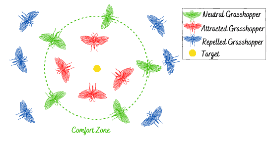
Let’s dig a little deeper into the strength of these social forces. When the distance between two grasshoppers is between ${[0, 2.079]}$ , repulsion occurs, and when the distance between two grasshoppers is ${2.079}$ , neither attraction nor repulsion occurs, which form a comfort zone. When the distance exceeds ${2.079}$ , the attraction force increases, then progressively decreases until it reaches ${4}$ .

The function ${s}$ fails to apply forces between grasshoppers when the distance between them is larger than ${10}$ . In order to solve this problem, we map the distance of grasshoppers in the interval ${[1,4]}$ . The graph below explains the social interaction in more detail:

4.2. Force of Gravity

Let’s now move forward to the second force, which is the force of gravity. The equation below shows how to calculate the force of gravity ${G_i}$ :

(5) $\begin{equation*} {G_i} = - g \hat{e_{g}} \end{equation*}$

where ${-g}$ represents the gravitational constant and $\hat{e_{g}}$ is unit vector toward center of earth.

4.3. Force of Wind Direction

Afterward, we investigate the force of wind direction, which greatly impacts the nymphs and adulthood grasshoppers. As a result, the movements of nymph and adulthood grasshoppers are correlated with the wind direction $\boldsymbol{A_i}$ . The equation below shows how to compute ${A_i}$ :

(6) $\begin{equation*} {A_i} = u \hat{e_{w}} \end{equation*}$

where ${u}$ represents the drift constant and $\hat{e_{w}}$ is the unit vector in the wind direction.

4.4. Grasshopper Position

Let’s reconstruct Equation 1 using Equations 3, 4, 5 and 6:

(7) $\begin{equation*} {X_i} = \sum_{j=1}^{N} s({d_{ij}}) \hat{d_{ij}} - g \hat{e_{g}} + u \hat{e_{w}} = \sum_{j=1}^{N} s({|{x_j} - {x_i}|}) \frac{|{x_j} - {x_i}|} {d_{ij}}} - g \hat{e_{g}} + u \hat{e_{w}} \text{ , where } {i} \neq {j} \end{equation*}$

In order to solve optimization issues and prevent grasshoppers from quickly reaching their comfort zone and the swarm from failing to converge to the target location (global optimum), we’ll make some modifications in Equation 7:

(8) $\begin{equation*} {X_{i}^d} = c ( \sum_{j=1}^{N} c \frac{UB_{d} - LB_{d}} {2} s({|{x_{j}^d} - {x_{i}^d}|}) \frac{|{x_j} - {x_i}|} {d_{ij}}}) + \text{Best Solution}} \text{ , where } {i} \neq {j} \end{equation*}$

where ${G = 0}$ , ${A}$ is the best solution in the $\text{d-th}$ dimension, and ${UB_{d}}$ and ${LB_{d}}$ are the upper and lower bounds in the $\text{d-th}$ dimension, respectively.

The parameter ${c}$ represents the decreasing coefficient, and it is in charge of decreasing the comfort zone, repulsion zone, and attraction zone. In order to balance the exploration and the exploitation phases using the grasshopper approach, the coefficient ${c}$ decreases according to the number of iterations. Here’s the model for ${c}$ :

(9) $\begin{equation*} {c} = {c_{max} - iter \frac{c_{max} - c_{min}}{Max_{iter}}} \end{equation*}$

where ${c_{max}}$ and ${c_{min}}$ are the maximum and minimum values of ${c}$ respectively, ${iter}$ is the current iteration, and ${Max_{iter}}$ is the maximum number of iterations.

5. Steps of GOA Algorithm

Let’s now take a look at the implementation of the GOA optimizer:

As we can see in the algorithm, we start by initializing the parameters { ${c_{max}, c_{min}, f, l, iter}$ } and the grasshopper population ${n}$ . Then, we evaluate each solution by calculating its value using the fitness function. After evaluating each solution in the population, we assign the best solution according to its value. Afterward, we update the coefficient parameter ${c}$ to shrink the attraction, repulsion, and comfort zones (Equation 9).

The function ${s}$ (Equation 4) divides the search space into repulsion, comfort, and attraction zones. As explained in Section 4.1, when the function ${s}$ fails to apply forces between the grasshoppers, we map the distance in the interval ${[1,4]}$ .

Then, we update each solution in the population based on the distance between the grasshopper (the solution) and the other grasshopper (the other solution). We also update the best solution in the population and the decreasing coefficient parameter ${c}$ using Equation 8.

In the case of a grasshopper violating the boundaries after updating the solution, we bring the grasshopper back to its domain. Then, we repeat the previous three steps for each solution in the population.

Afterward, we update and evaluate each solution to assign the best one in the population. We repeat the overall operations until we reach ${Max_{iter}}$ the maximum number of iterations to return the best global solution.

It is worth noting that the time complexity of the grasshopper algorithm is generally related to the number of iterations and the number of agents. So, $\boldsymbol{{O}({n} \times {Max_{iter}})}$ represents the time complexity of this algorithm with $\boldsymbol{n}$ is the number of agents and $\boldsymbol{Max_{iter}}$ is the number of iterations.

6. Numerical Example of Grasshopper Optimization Algorithm

To understand the grasshopper optimizer algorithm, we use a numerical example.

6.1. Initialization

Firstly, we randomly initialize the population of grasshopper ${X_i}$ $\text{(i=1, 2,..., n)}$ , where ${n = 4}$ . Afterward, we initialize all the parameters ${Max_{iter}}, {c_{max}}, {c_{min}}, {LB}, {UB}$ , and ${d}$ using a random set of values:

$\left\{ \begin {array} {llllll} { Max_{iter} = 9} \text{ , Maximum number of iterations} \\ { c_{max} = 1 } \text{ , Maximum value of c} \\ { c_{min} = 0.00004 } \text{ , Minimum value of c } \\ { LB = -5 } \text{ , Lower bound} \\ { UB = 5 } \text{ , Upper bound} \\ { d = 2 } \text{ , Dimension} \\ \end{array}$

6.2. Compute the Fitness Value

Here’s the fitness function in order to calculate the fitness value for each grasshopper:

$Fitness Function= 4 \times {X(1)^2} - 2.1 \times {X(1)^4} + \frac{1}{3} \times {X(1)^6} + {X(1)} \times {X(2)} - 4 \times {X(2)^2} + 4 \times {X(2)^4}$

Let’s calculate the fitness value for each grasshopper in the current population using the fitness function:

6.3. Optimal Solution and Check the Condition

After calculating all the fitness values, we have to select the optimal solution among all. The optimal solution is the one that has the smallest fitness value across all grasshoppers. As a result, ${Fitness = 166.9550}$ is the best solution for the first iteration. Let’s move forward to check the $\emph{while}$ condition. Notice that the number of iteration ${Max_{iter} = 9}$ and the ${\text{current iteration} = 2}$ , which means condition true ${(2 < 9)}$ . As a result, we move to the next step.

6.4. Normalization of the Distance

We need to compute ${c}$ in order to normalize the distance between grasshoppers using the equations below:

(10) $\begin{equation*} \sum_{j=1, {i} \neq {j}}^{N} c \frac{UB_{d} - LB_{d}} {2} s({|{x_{j}^d} - {x_{i}^d}|}) \frac{|{x_j} - {x_i}|} {d_{ij}}} \end{equation*}$

(11) $\begin{equation*} {c} = {c_{max} - iter \frac{c_{max} - c_{min}}{Max_{iter}} = 1 - 2 \times \frac{1 - 0.00004}{9} \approx 0.80001} \end{equation*}$

Here’s the result of normalizing the distance between grasshoppers:

6.5. Update Position

To update the position for each grasshopper using Equation 8, we require the current position of the grasshopper (calculated in section 6.2), the best solution found (calculated in section 6.3), and other grasshopper positions (calculated using the distance in section 6.4). Here’s the new position for grasshoppers:

We got the values of the new position by adding the best solution found ${(X(1), X(2))}$ to ${c \times (Distance(1), Distance(2)) }$ .

6.6. Compute the New Fitness Value

Before computing the new fitness value, we bring the current grasshopper back if it goes outside boundaries ${[LB, UB] = [-5, 5]}$ . The table in section 6.5 shows that all grasshoppers are within the boundary. So, let’s now compute the new fitness values for each grasshopper in the current population:

6.7. Best Global Solution

We check if there’s any new best solution to update the best solution. To do that, we compare the old fitness value with the new fitness value for each grasshopper. After comparing the old and the new fitness values ${(141.9027 < 166.9550)}$ , we update the $\text{best solution = 141.9027}$ and we increment the counter. Then, we repeat the ${while}$ until reaching ${ iter = {Max_{iter} = 9}$ . If ${iter = {Max_{iter}} = 9}$ then stop the ${while}$ && return the $\text{best global solution = 124.3374}$ . The fitness values for each iteration are presented in the tables below:

7. Advantages and Disadvantages of GOA Algorithm

Same as any optimizer algorithm, the GOA algorithm has its benefits and drawbacks. Let’s then take a look at the benefits and drawbacks of the GOA algorithm:

8. Conclusion

In this article, we discussed the grasshopper optimization algorithm using a numerical example to unlock its mechanism. This algorithm searches for an optimal global solution to a problem using the swarm population in nature. We introduced this algorithm because it’s highly effective in solving global unconstrained and constrained optimization issues.

Full Archive

About Baeldung

Core Concepts

Operating Systems

Artificial Intelligence

Graph Theory

Latex