Yes, we're now running our only Summer Sale. All Courses are 30% off until 20th July, 2026:
Whale Optimization Algorithm
Last updated: April 30, 2023

Learn through the super-clean Baeldung Pro experience:
>> Membership and Baeldung Pro.
No ads, dark-mode and 6 months free of IntelliJ Idea Ultimate to start with.
1. Overview
In this tutorial, we’ll go over what the Whale Optimization Algorithm (WOA) is and what it does. Furthermore, we’ll go over the algorithm and use an example to demonstrate how WOA would solve some simple optimization.
2. What Is the Whale Optimization Algorithm?
WOA is a meta-heuristics algorithm. As implied by the name, this algorithm was proposed for optimizing numerical problems by Mirjalili and Lewis, 2016. The inspiration for WOA comes, in particular, from the social behavior and the bubble-net hunting of humpback whales in oceans.
3. Who Are the Humpback Whales?
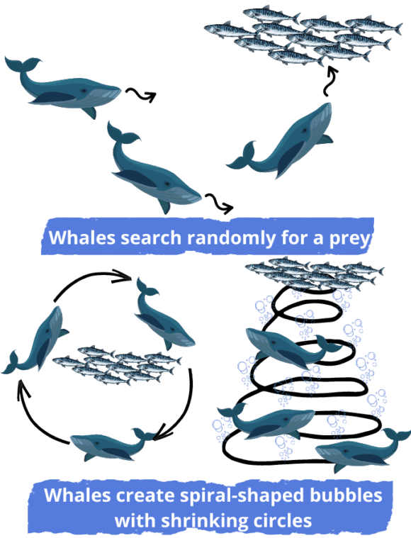
Humpback whales are among the largest mammals in the world. They are also one of seven different types of whales. It also has a one-of-a-kind hunting mechanism known as the bubble-net feeding method. They are unquestionably intelligent because their brains contain spindle cells. This foraging behavior is accomplished by the formation of special bubbles in the form of a spiral or path. As a result, let’s investigate the whale leadership hierarchy:
- The leader whale finds the prey and dives down for about 12 meters approximately, creating a spiral-shaped bubble around the prey, and then swimming up to the surface while following the bubbles
- An experienced whale who support the leader by making a call to synchronize
- The others form a formation behind the leader and take the same position for each lunge
In short, the bubble-net hunting of humpback whales may resemble the image below:
4. Mathematical Model of the Whale Optimization Algorithm
The WOA algorithm imitates the social behavior and hunting method of humpback whales in oceans. So, let’s go over the fundamentals of whale hunting:
- Exploration phase: search for the prey
- Encircling the prey
- Exploitation phase: attacking the prey using a bubble-net method
Let’s take a look at the mathematical model behind each phase of the whale hunting process.
4.1. Exploration Phase: Searching Model
The search agent (humpback whale) looks for the best solution (the prey) randomly based on the position of each agent. We update the position of a search agent during this phase by using a randomly selected search agent rather than the best search agent. Following that, if  , as defined in Equation 3, then force the search agent to move away from a reference whale. Here’s the mathematical model behind this phase:
(1) 
(2) 
Where  is a random position vector selected from the current population, and {
 ,
,  } are coefficient vectors. Besides, here are the equations of { and } that can be used to find the best search agents:
(3) 
(4) 
Where  is a random vector in range [0, 1] and
  decreases linearly from 2 to 0 during the iterations.
4.2. Encircling Model
Humpback whales encircle the prey during hunting. Then, they consider the current best candidate solution as the best solution and near the optimal one. In short, here’s the model of encircling behavior that is used to update the position of the other whales towards the best search agent:
(5) 
(6) 
Where t is the current iteration,  is the position of the best solution,
  refers to the position vector of a solution, and {, } are coefficient vectors as shown in Equations 3 and 4.
4.3. Exploitation Phase: Bubble-Net Attacking Model
This phase focuses on using a bubble-net to attack the prey. This bubble-net strategy combines two approaches. Let’s look at the mathematical model of each approach in order to better understand this step:
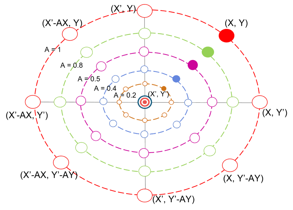
- Shrinking encircling mechanism: The value of in this mechanism is a random value within the [-a, a] interval, and the value of decreases from 2 to 0 over the course of iterations, as shown in Equation 3. Let’s now define random values for in [-1, 1]. We can also define the new position of a search agent anywhere between the current best agent’s position and the agent’s original position. So, let’s look at the graph that displays the possible positions from
 to
to  :
:
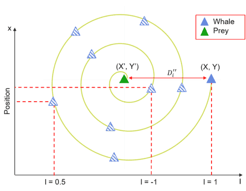
- Spiral updating position mechanism: This method starts with the calculation of the distance between the whale and the prey . Here’s the spiral equation behind the helix-shaped movement of humpback whales to define the position between whale and prey:
(7) 
Where  represents the distance between the whale and the prey (best solution obtained so far),
  is a random number between [-1, 1], and
  is a constant defining the shape of the logarithmic spiral. Let’s now define the mathematical model behind the humpback whale’s swimming style around the prey using a shrinking circle and also following a spiral-shaped path at the same time:
(8) 
Where  represents the probability of selecting one of these two methods to update the position of whales. Next, let’s say that the probability of choosing between the two approaches is 50%. Then, is a random number in [0, 1]. Here’s the graph that explains the spiral updating position in more detail:
5. Flowchart of a Whale Optimization Algorithm
Let’s take a look at the flowchart:
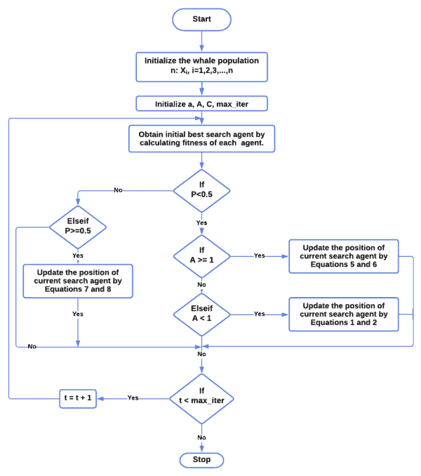
First, we must initialize the whale population  as well as the values. Then, we evaluate the fitness solution value of the search agent. Next, we set the number of iterations to 1. Afterward, we use Equation 1 to search for prey. Then, we encircle it using Equation 5, after finding the prey. Following that, we update the position of search agents to attack the prey using the bubble-net strategy in Equation 8. Then, we update the values of {
 ,
,  ,
,  } with the new position of the search agent. Afterward, we check the constraints of equality and inequality of and
  for the new position of each search agent and then increase the iteration number.
Finally, if we reach the maximum number of iterations  , we’ll stop and save the fitness value as the best solution; otherwise, we’ll repeat the process until we find a solution.
6. Explanation of Whale Optimization Algorithm With Example
Let’s discover a simple example to understand the whale optimization algorithm:
- Step 1: First, let’s randomly initialize the population of whales


- Step 2: Then, we initialize the iteration counter t = 0
- Step 3: Next, let’s initialize the value of a=2 (because it decreases from 2 to 0) and {
 } using a random values (based on the equations 3 and 4), and let’s define
  :
:
![\[{a} = 2 - t * \frac{2}{max\_iter}\]](/wp-content/ql-cache/quicklatex.com-fbdac2f00c90c7140f966d3e43af3664_l3.svg "Rendered by QuickLaTeX.com")
- Step 4: Afterward, we need to evaluate each search agent
 by calculating its fitness function
  . Here’s the fitness function example:
![\[Fitness = 4 {X(1)^2} - 2.1 {X(1)^4} + \frac{1}{3} {X(1)^6} + {X(1)}{X(2)} - 4 {X(2)^2} + 4 {X(2)^4}\]](/wp-content/ql-cache/quicklatex.com-109ae6974dde06349a2601fac80343d7_l3.svg "Rendered by QuickLaTeX.com")
Here’s the result of the fitness function after setting a random initialization of the population for five search agents:
| Sr. No | X(1) | X(2) | Fitness |
|---|---|---|---|
| 1. | -1.5002 | -1.4834 | 16.0964 |
| 2. | -3.0340 | 3.3083 | 1.4945 |
| 3. | -2.4892 | 0.8526 | 2.1752 |
| 4. | 1.1604 | 0.4972 | 1.4192 |
| 5. | -0.2671 | 4.1719 | 2.4043 |
As a result, the optimal solution is the one with the lowest fitness value of all search agents. Thus,  is the optimal solution for the first iteration.
- Step 5: Let’s now update the position vector according to and
 :
:
![\[\left\{ \begin {array} {ll} \text{if } {p \ge 0.5} \text{, update by Equations 7 and 8 }\\ \text{if } {p<0.5} \left\{ \begin {array} {ll} \text{if } {A \ge 1 } \text{, update by Equations 5 and 6 } \\ \text{if } {A < 1 } \text{, update by Equations 1 and 2 } \end{array} }\]](/wp-content/ql-cache/quicklatex.com-4d64735b8749ee455ed87f09d5a9ec24_l3.svg "Rendered by QuickLaTeX.com")
- Step 6: If
 then update values {
 } && repeat steps 4 and 5
 - Step 7: If
 then return the best solution
7. Conclusion
In this article, we discussed the whale optimization algorithm, and how understanding this algorithm can facilitate the search for an optimal solution to a problem using the way of whales. We introduced this algorithm because it is highly effective while remaining simple enough to be easily understood.