

Yes, we're now running our only Summer Sale. All Courses are 30% off until 20th July, 2026:
Learn through the super-clean Baeldung Pro experience:
>> Membership and Baeldung Pro.
No ads, dark-mode and 6 months free of IntelliJ Idea Ultimate to start with.
1. Introduction
Computer networks consist of intricate communication systems that enable us to exchange data worldwide. But, transmitting data through a computer network includes processing it with several network functions, leading it from a source to a destination point. In particular, we call the process of selecting a path that data goes through to reach its destination of routing.
In this tutorial, we’ll learn about dynamic routing, focusing on distance vector- and link state-based strategies. First, we’ll briefly review the routing process, from basic concepts to categories. So, we’ll understand dynamic routing by defining its classes of distance vector and link state. Finally, we’ll review the studied concepts and compare the dynamic routing classes in a systematic summary.
2. Routing
In short, we can define the routing process as the transmission paths in a computer network to make a given data reach its destination. However, it is not a simple process. As a result, we have different routing categories and algorithms, each with particular benefits and shortcomings.
The first routing category is static routing. In such a category, routing tables (tables with all available routes in a router) are manually defined. In practice, it means that the network operators set up all the routing table entries of a static router. We commonly use static routers with networks in which connections and data transmission parameters are known and do not vary much.
A sub-category of static routing consists of default routing. Routers adopt a default route when it does not have any precise routing entry that fits a data transmission. However, some routers can use the strategy of only having a default route: the default routing. We can use it, for example, when a router is directly connected to an Internet Service Provider.
Finally, we have the category of dynamic routing. In this case, the routers create and update routing tables in runtime and based on the network conditions. For instance, dynamic routers can adapt their routers if a link goes down or gets overloaded. There exist two classes of dynamic routing: distance vector-based and link state-based. We’ll discuss these classes in the following sections.
3. Distance Vector
Distance vector-based dynamic routing considers that the best path between two entities communicating with each other is the shortest one. In this case, distance does not represent physical distance but hops, typically. A hop is, in short, a device that processes the network traffic before it reaches its destination.
However, it is relevant to highlight that we can use other metrics to measure distance and determine the shortest routing path, such as delay.
A distance vector-based router communicates and evaluates paths only between them and their immediate neighbors. So, routers share their information about the network with their neighbors, enabling them to calculate the distance between them and a particular destination.
Let’s consider that the distance metric is hops, and there is a packet in router R1 that must reach server S, as depicted next:
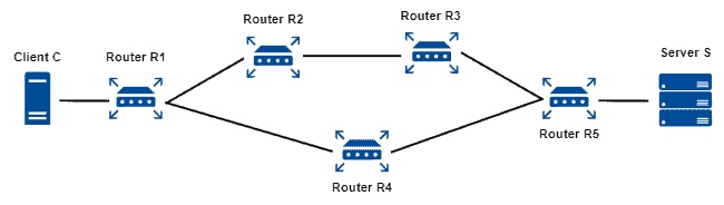
With a hop-based routing strategy, R1 will choose the path through the router R4 since it will result in two hops until the packet reaches the destination. On the other hand, if router R1 selected router R2, it would result in three hops until the packet reaches its destination, which is not the best option in such a scenario.
A problem related to distance vector-based routing is that updating routing tables is a slow process. So, bad news typically takes a long time to reach some routers, and the convergence time (time to a router producing an updated routing table) is long. Furthermore, there are loop-sensitive protocols.
3.1. Distance Vector-based Protocols
The most popular distance vector-based routing protocol is the Routing Information Protocol (RIP). In summary, it defines a periodic update time for a router to update its table, broadcasting (V1) or multicasting (V2) the updated to its neighbors. The RIP protocol defines a series of timers to control a router’s lifecycle: update, invalidation, hold down, and flush. These timer helps the routers to keep their tables valid and with recent information.
4. Link State
Link state routing protocols have a broad perspective of the network instead of working with the state of the neighbors’ routers, like distance vector routing protocols. To keep track of the state of the entire network, the routers using link state-based protocols have three tables:
- Route Table: sometimes called Forwarding Database, the routing table defines the network traffic forwarding rules of a given router
- Topology Map: also called Link State Database, this table holds topological information about the working network
- Neighbors Table: sometimes referred to as Adjacency Database, it keeps data and routing details about directly connected neighbors of a given router
For building these tables, we can summarize the operation of link state-based routers in four simple steps:
- Discover the neighbor routers by sending and receiving hello messages. It will enable a particular router to build its neighbor table
- Measure the costs to communicate with an adjacent router, thus flooding the information to the network domain; routers repeat such a process (fully or partially) every time the network changes, flooding update messages
- Receive route updates from other routers. So, the routers can build and maintain the topology map of the network
- Build a logical tree with the current router as the root. Thus, the router can execute shortest-path first algorithms (typically Dijikstra) to allocate the paths with the lowest cost for all the possible destinations in its routing table
Link state-based routers can employ different metrics to determine the shortest path to a destination. For example, they can adopt bandwidth, delay, or jitter as the optimization criteria.
Let’s consider the same example of the previous section, where there is a packet in router R1 that must reach server S. However, now we have the information about the transmission delay between the connected entities:
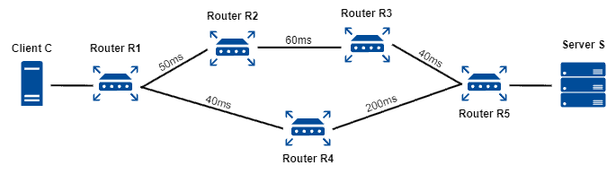
With a minimum delay-based routing strategy and knowing the state of the entire network, R1 will choose to send the network traffic to R2, which in turn will send it to R3, then to R5, and finally reach the destination. The described path results in a total delay of 150ms. The alternative path, from R1 to R4 and then R5, results in a total delay of 240ms, making it a worse option.
The major problem with link state-based routing protocols is that it generates heavy control traffic due to the routers flooding updates in the network. Furthermore, these flooding events can create transmission loopings, which make the overloading problem even worse. However, we can mitigate these looping problems by properly configuring the packets’ Time To Live (TTL) field.
4.1. Link State-based Protocols
The most known link state-based protocols are called Open Shortest Path First (OSPF) and Intermediate System to Intermediate System (IS-IS). Both protocols implement the basics of link state-based routing, as previously described in this section. Moreover, they have other relevant similarities, such as being interior gateway protocols (exchange data between gateways of a single autonomous system, such as between local networks of a corporation), providing authentication methods, and supporting an unlimited number of hops count to route a packet.
However, these protocols also present some differences. Examples are that OSPF runs on the network layer and IS-IS runs on the data link layer; OSPF supports working with virtual links and IS-IS does not; and OSPF identifies routers through the Router ID while IS-IS uses a System ID.
5. Systematic Summary
Routing is essential for enabling data exchange through the current computer networks. One of the categorizations of routing protocols refers to which strategy to use for deciding which route is the best: distance vector and link state.
Distance vector-based routing protocols decide the shortest path based on a local view of the neighbors of a given router. In this scenario, the most common metric is the number of hops to the destination.
Link state-based protocols, in turn, choose the best route using a predefined criterion (such as delay or bandwidth). Each router considers a global view of the routers in a network.
The following table summarizes and compares relevant characteristics of distance vector- and link state-based routing:
| Distance Vector | Link State | |
|---|---|---|
| Network View | Based on the neighbors’ routers | Based on all the routers working in a network |
| Working Tables | Route table | Route table, topology map, and neighbors table |
| Tables Update | Based on routing tables | Based on link states |
| Update Frequency | Periodic | Triggered |
| Convergence Time | Slower than link state-based protocols | Faster than distance vector-based protocols |
| Bandwidth Usage | Moderate | Intensive |
| Protocol Examples | RIP | OSPF and IS-IS |
6. Conclusion
In this tutorial, we studied the two categories of dynamic routing protocols: distance vector and link state. First, we briefly reviewed the routing process. Thus, we particularly investigated the categories of distance vector- and link state-based protocols. Finally, we outlined the main concepts and compared such routing protocol categories in a systematic summary.
We can conclude that routing is a critical task for modern networking. However, we can not definitely point out the best routing protocol among the explored ones. The choice of a specific protocol depends on the complexity of the network and the available resources.