The Rod Cutting Problem in Computing

1. Introduction

In this tutorial, we’re going to see what the Rod Cutting Problem is and then explore a few different ways that we can solve it.

2. What Is the Rod Cutting Problem?

Imagine we have a rod of length n. We can cut this rod into arbitrary lengths and sell those cut lengths. We also have a table of prices for different lengths of cut rods. We aim to determine the lengths to cut the rod into for the maximum price.

For example, if we have a rod of length 4m, and we have a pricing table of:

This means that we have several different ways that we could cut this up and sell it:

• Four different pieces of 1m each – total price $4
• Two different pieces of 2m each – total price $10
• One piece of 4m – total price $9
• One piece of 1m and one piece of 3m – total price $9
• Two pieces of 1m and one piece of 2m – total price $7

With a rod of this length, we can easily enumerate the options by hand and see the best answer. Here we can see that by cutting our rod into two pieces of length 2m, we can get a total price of $10. Every other combination gives a lower price, so we can see that this is the optimal answer.

However, if we have a much longer rod, with many more combinations of how we can cut it up, this becomes much harder to solve.

3. Recursive Solution

The most obvious solution is a simple recursive one. Given our rod, we’ll iterate along every step, see the price if we cut it here, and simply return whichever value is highest. The price for each point is done by looking up the price for cutting at this point and recursively calling our algorithm on the amount remaining:

algorithm cutRod(prices, length):
    // INPUT
    //    prices = an array of prices
    //    length = the total length of the rod
    // OUTPUT
    //    Returns the maximum revenue obtainable by cutting up the rod and selling the pieces.

    if length = 0:
        return 0

    result <- 0
    for l in 1 to length:
        thisCut <- prices[l] + cutRod(prices, length - l)
        result <- max(result, thisCut)
    
    return result

For example, given our prices and a 4m rod, we would:

• Check at position 1 – this will come to $1 + the best price for cutting a 3m rod
• Check at position 2 – this will come to $5 + the best price for cutting a 2m rod
• Check at position 3 – this will come to $8 + the best price for cutting a 1m rod
• Check at position 4 – this will come to $9 + the best price for cutting a 0m rod

Every step in this is calling back into our algorithm with a shorter rod until the remaining rod is 0m long, at which point we stop.

This works and is relatively easy to understand. However, the complexity will grow exponentially. The time complexity is O(2^n). So if we have 4m rods, this will take 2^4 = 16 iterations. And being exponential, this gets big fast. A 10m rod will take 1,024 iterations, for example.

4. Memoized Recursive Solution

One way that we can improve our recursive solution is by the use of memoization. This is a technique whereby we remember the results of a given input, so we can reuse it if we see the same input again.

Let’s look at a tree of the possible rod lengths:

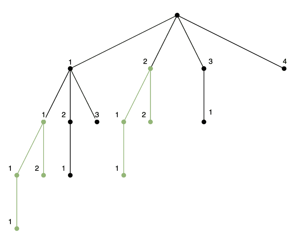
If we look carefully, we’ll see two identical sub-trees here – those highlighted in green. We don’t need to calculate both of these and can re-use the result for one when we get to the other. The bigger the tree – the longer our original rod – the more nodes we can trim in this way.

In order to do this, we can use a variation of the previous algorithm. Every time we finish calculating the best price for a given rod length, we can record this against that length. Then, if we see another call for a rod of a previously calculated length, we can reuse the same score instead of doing all the work again.

algorithm cutRodMemoized(prices, length, memory):
    // INPUT
    //    prices = an array of prices
    //    length = the total length of the rod
    //    memory = the rray to store results of subproblems
    // OUTPUT
    //     Returns the maximum revenue obtainable by cutting up the rod and selling the pieces.

    if memory[length] != null:
        return memory[length]

    if length = 0:
        return 0

    result <- 0
    for l in 1 to length:
        thisCut <- prices[l] + cutRod(prices, length - l, memory)
        result <- max(result, thisCut)
    
    memory[length] <- result
    return result

Our previous attempt had exponential complexity. This one, instead, has quadratic complexity of O(n^2) at worst. This means that it might be worse for very small rods – a rod of length 3m will have a time complexity of 9 compared to 8 before. This is because of the extra work needed in storing and checking our record of rod prices. However, a rod of length 10m will have a time complexity of 100 here, compared to 1,024 before, because we’re doing notably less work due to the trimming of nodes.

However, this comes at a cost in space complexity. The previous algorithm did not need to store any state, whereas this one will need to store up to one value for each possible rod length, giving it a space complexity of O(n).

5. Dynamic Programming Solution

Another option we have is to leverage dynamic programming. This is a technique whereby a problem is broken down into smaller problems that are themselves optimized.

In this case, we can split our problem into two parts. We iterate over our rod in units and calculate the price of cutting the rod here plus the best price for what’s remaining. This sounds the same as our earlier algorithm, except we can do it iteratively by storing the values as we go.

So how does this work? We iterate over every possible rod size up to the size we’re working with, calculate the best solution for a rod of that size and store it. We can then use these previously stored solutions in our next iteration instead of doing the work again:

algorithm cutRodDP(prices):
    // INPUT
    //    prices = an array of prices
    // OUTPUT
    //    Returns the maximum revenue obtainable by cutting up the rod and selling the pieces.

    bestPrices <- array of size prices.length + 1, initialized with 0
    
    for rodLength in 1 to prices.length:
        bestPriceForRodLength <- 0
        for cutLength in 1 to rodLength:
            possiblePrice <- prices[cutLength] + bestPrices[rodLength - cutLength]
            bestPriceForRodLength <- max(bestPriceForRodLength, possiblePrice)
            bestPrices[rodLength] <- bestPriceForRodLength
    
    return bestPrices[prices.length]

This seems daunting, so let’s look at a worked example.

We start by calculating the best possible price for a rod of length 1m. There’s nowhere that we can cut this rod, so the answer is simply $1.

Next, we calculate the best possible price for a rod of length 2m:

• If we cut it after 1m, we get the calculated best price for this 1m – $1 – plus the price from our table for the remaining 1m – $1. This means we get a total price of $2
• If we don’t cut it, we get the price from our table for the 2m – $5

This means we can see that the best price for a rod of length 2m must be $5.

Next, we calculate the best possible price for a rod of length 3m:

• If we cut it after 1m, we get the calculated best price for this 1m – $1 – plus the price from our table for the remaining 2m – $5. This means we get a total price of $6
• If we cut it after 2m, we get the calculated best price for this 2m – $5 – plus the price from our table for the remaining 1m – $1. This means we get a total price of $6
• If we don’t cut it, we get the price from our table for the 3m – $8

This means we can see that the best price for a rod of length 3m must be $8.

Finally, we calculate the best possible price for a  rod of length 4m:

• If we cut it after 1m, we get the calculated best price for this 1m – $1 – plus the price from our table for the remaining 3m – $8. This means we get a total price of $9
• If we cut it after 2m, we get the calculated best price for this 2m – $5 – plus the price from our table for the remaining 2m – $5. This means we get a total price of $10
• If we cut it after 3m, we get the calculated best price for this 3m – $8 – plus the price from our table for the remaining 1m – $1. This means we get a total price of $9
• If we don’t cut it, we get the price from our table for the 4m – $9

Because this is the full length of the rod, we can now see that $10 is the best price we can get.

Perhaps unsurprisingly, this has essentially the same time and space complexity as our memoized solution. This is because this is effectively the same algorithm only in iterative rather than recursive form.

6. Conclusion

In this article, we’ve seen the Rod Cutting problem and then looked at a few ways to solve it. We’ve also seen the complexities of these solutions to understand better which solution to select in a given scenario.