Yes, we're now running our only Summer Sale. All Courses are 30% off until 20th July, 2026:
Random Sample Consensus Explained
Last updated: February 13, 2025

Learn through the super-clean Baeldung Pro experience:
>> Membership and Baeldung Pro.
No ads, dark-mode and 6 months free of IntelliJ Idea Ultimate to start with.
1. Introduction
In this tutorial, we’ll explore the Random Sample Consensus (RANSAC) algorithm. It describes a method to detect outliers in a dataset using an iterative approach.
2. Motivation
Outliers appear in datasets for various reasons, including measurement errors and wrong data entry. They may also be inherent to the data at hand.
2.1. An Example
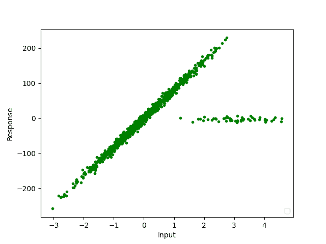
In the data shown we see a typical dataset encountered i.e. in signal processing:
The outliers are easy to spot visually, we mark them in purple:
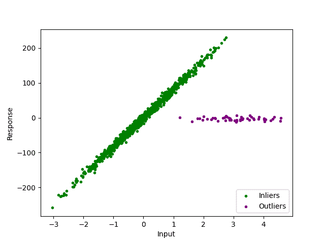
In this example, it’s easy to see the outliers. In other cases, we might not even be able to visualize them in two dimensions. Furthermore, we certainly want an algorithm that detects our outliers rigorously and automatically.
2.2. Further Processing
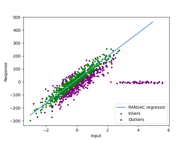
We can also see that the outliers prevent us from further data processing. As an example, we have a look at a linear regression:
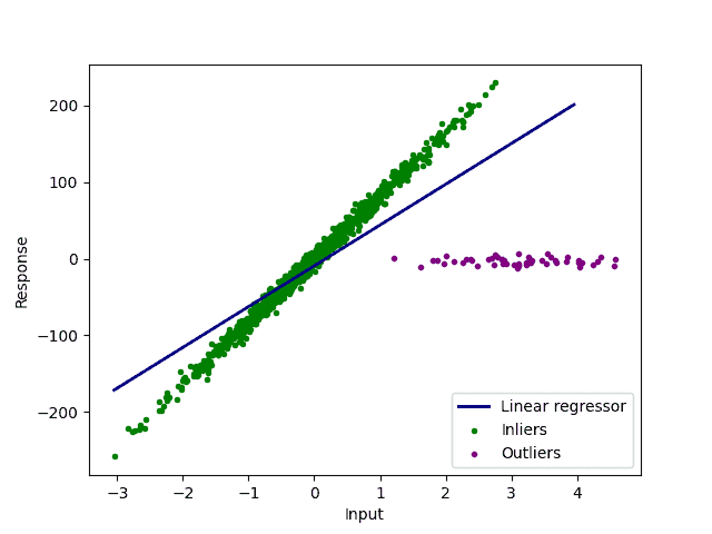
As we can see, the linear regression fails to describe our data correctly.
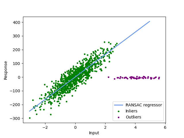
What we do want in this example is a linear regression, that only goes through our inliers:
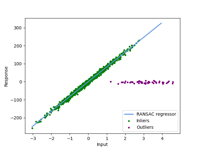
3. Eliminating Outliers With the RANSAC Algorithm
To detect our outliers correctly and to build a model that ignores them in computation, we use the RANSAC algorithm. It works by taking a random subset of our given data and creating a model from it. Then we check how well the whole dataset fits the model. We repeat these steps until we have found a model that fits our data well. In this process, we mark all points that are not close to it as outliers.
3.1. The Implementation
Let’s take a closer look at the algorithm:
algorithm RANSAC(n, m, data, t, k):
    // INPUT
    //    n = number of inliers we use in each iteration
    //    m = maximum number of iterations
    //    data = input data
    //    t = threshold for determining a good fit
    //    k = number of close points required for a good model fit
    // OUTPUT
    //    bestFit = the best model found

    i <- 0
    bestFit <- null
    bestError <- infinite

    while i < m:
        tempInliers <- selectRandom(data, n)
        tempInliersAdd <- an empty list
        tempModel <- fit(tempInliers)

        for point in data:
            if point not in tempInliers:
                if distance(point, tempModel) < t:
                    tempInliersAdd.add(point)

        if length(tempInliersAdd) > k:
            newModel <- fit(tempInliers and tempInliersAdd)
            if newModel.error > bestError:
                bestError <- error
                bestFit <- newModel

    return bestFit
In the center of the algorithm is our “for” loop. In this loop, we select a random subset of our data, having the previously chosen size  . For this data, we fit our model. This can be any kind of model, for example, a simple linear regression.
After fitting the model, we check how far away all the other points from our original dataset are with respect to the model in our second for loop. For this distance, we use the parameter  as a threshold. From these points, we create a new List, called tempInlierAdd.
If this list has a size larger than our parameter  , we can consider it as a candidate for an appropriate model. Then we create a model from tempInlier and tempInlierAdd and compare it to the best model from our previous iterations.
3.2. Model Parameters – Threshold
To determine how far how away from our fitted line our points can be to still consider them as inliers, we use the parameter as a threshold:
If our threshold is chosen too small, as in our picture, we may detect too many points as inliers. In most RANSAC implementations, the threshold is calculated as the median of y-values from our dataset. If no threshold is given by the user. Changing the threshold manually in our example yields a much more reasonable outlier classification:
A wrong threshold can not only detect the wrong outliers, but it can also result in a wrong data model. Thus, it is essential to choose it correctly.
3.3. Model Parameters – Number of Iterations
The higher the number of iterations, the higher the probability that we detect a subset without any outliers in it. We can use a result from statistics, that uses the ratio of inliers to total points  , the number of data points we need for our model calculation and the probability
  that we encounter a subset without outliers in it:
![\[k={\frac {\log(1-p)}{\log(1-w^{n})}}\]](/wp-content/ql-cache/quicklatex.com-c4ac75e04dc5e0b987f98da6de22ce92_l3.svg "Rendered by QuickLaTeX.com")
As we can see with a simple example of  ,
,  and
and  , we need roughly 41 iterations to obtain a model without outliers with a probability of 99%.
4. Advantages and Alternatives
As we have seen in our formula above, our RANSAC algorithm is only fast and correct, if the model that we want to fit, i.e. the linear regression, needs a small number of points. Additionally, the number of outliers must be limited, if we do have more than 50% outliers we may run into problems.
Besides the RANSAC algorithm, there exists a variety of methods to detect outliers. For example, classification algorithms such as the support vector machine (SVM). In the case of a linear SVM, we use a simple line to divide our dataset into inliers and outliers. We achieve this meaningfully by maximizing the cumulative distance between our line and our points from the dataset. Since we only want to divide our set into two classes, inliers and outliers, we use a 1-class SVM algorithm. Another notable method is the k-nearest neighbor algorithm (kNN).
5. Conclusion
In this article, we discussed the structure and implementation of the RANSAC algorithm. We also had a look at its pros and cons and viable alternatives.