

Learn through the super-clean Baeldung Pro experience:
>> Membership and Baeldung Pro.
No ads, dark-mode and 6 months free of IntelliJ Idea Ultimate to start with.
Last updated: February 12, 2025
Learn through the super-clean Baeldung Pro experience:
>> Membership and Baeldung Pro.
No ads, dark-mode and 6 months free of IntelliJ Idea Ultimate to start with.
Many deep-learning frameworks provide us with intuitive interfaces to set the layers, tune the hyper-parameters and evaluate our models. But to discuss the results properly, and more importantly, to understand how the networks work, we need to be familiar with fundamental concepts.
In this tutorial, we’ll talk about Backpropagation (or Backprop) and Feedforward Neural Networks.
Feedforward networks are the quintessential deep learning models. They’re made up of artificial neurons that are organized in layers.
A neuron is a rule that transforms an input vector  into the output signal we call the activation value
  :
:
(1) 
where  is the neuron’s bias, the
  are the weights specific to the neuron, and
  is the activation function such as ReLU or sigmoid. For example, here’s how the
  -th neuron in a layer computes its output after receiving two input values::

A layer is an array of neurons. A network can have any number of layers between the input and the output ones. For instance:
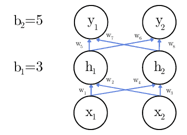
In the image,  and
and  denote the input,
  and
and  the hidden neuron’s outputs, and
  and
and  are the output values of the network as a whole. The values of the biases
  and
and  will be adjusted during the training phase.
The defining characteristic of feedforward networks is that they don’t have feedback connections at all. All the signals go only forward, from the input to the output layers.
If we had even a single feedback connection (directing the signal to a neuron from a previous layer), we would have a Recurrent Neural Network.
Let’s suppose we want to develop a classifier for detecting if there’s a dog in an image. To keep things simple, we’ll pretend that we can do that by inspecting only the values of two grey-scale pixels  and
and  (
(![x_1, x_2 \in [0, 255]](/wp-content/ql-cache/quicklatex.com-7fbfb38473f312616fa624aeeb38a367_l3.svg "Rendered by QuickLaTeX.com") ).
).
Let’s say that the network has only one hidden layer and that the inputs are  and
and  . Also, let’s suppose we use the identity function
  as the activation function:
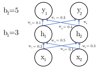
To calculate the activation value  , we apply the formula (1):
(2) 
Since we’re using the identity function as :
(3) 
We do the same for  ,
,  , and
, and  . For the latter two, the inputs are the values of and .
When training a neural network, the cost value  quantifies the network’s error, i.e., its output’s deviation from the ground truth. We calculate it as the average error over all the objects in the training set, and our goal is to minimize it.
For example, let’s say we have a network that classifies animals either as cats or dogs. It has two output neurons and , where the former represents the probability that the animal is a cat and the latter that it’s a dog. Given an image of a cat, we expect  and
and  .
.
However, if the network outputs  and
and  , we can quantify our error on that image as the squared distance:
(4) 
We compute , the cost for the entire dataset, as the average error over individual samples. So, if ![\widehat{\mathbf{y}}_i=[\hat{y}_{i, 1}, \hat{y}_{i, 2}, \ldots, \hat{y}_{i, m}]](/wp-content/ql-cache/quicklatex.com-963d8b4851b39ba310ec349ce3e6a226_l3.svg "Rendered by QuickLaTeX.com") is the ground truth for the
is the ground truth for the  -th training sample (
 ), and
 ![\mathbf{y}_i=[y_{i,1}, y_{i,2}, \ldots, y_{i,m}]](/wp-content/ql-cache/quicklatex.com-ff5758a5a4b57d4b6c83241d9dcbe4b8_l3.svg "Rendered by QuickLaTeX.com") is our network’s output, the total cost is:
is our network’s output, the total cost is:
(5) 
We use the cost to update the weights and biases so that the actual outputs get as close as possible to the desired values. To decide whether to increase or decrease a coefficient, we calculate its partial derivative using backpropagation. Let’s explain it with an example.
Let’s say we have only one neuron in the input, hidden, and output layers:
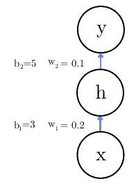
where is the identity function.
To update the weights and biases, we need to see how reacts to small changes in those parameters. We can do that by computing the partial derivatives of with respect to them. But before that, let’s recap how the variables in our problem are related:
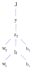
So, if we want to see how changing  affects the cost function, we should compute the partial derivative by applying the chain rule of Calculus:
(6) 
In this example, we’ll solve Equation (6), focusing only on the weight  to show how the calculation goes, but the method is the same for the other weight and the biases.
First, we calculate how the cost function varies with the output:
(7) 
Then, we need to calculate how the output value is affected by small changes in  . For this, we find the derivative of the activation function. Since we chose the identity function as activation function, the derivative is 1:
(8) 
Now, the only term missing is the partial derivative of with respect to the weight. Since  , the partial derivative will be:
(9) 
Now we have all the terms and we can calculate how the cost function is affected by a change in the weight :
(10) 
Let’s suppose that, at a certain moment during training, we have  , the desired output
  , and the current output
  . Using backpropagation, we compute the partial derivative of :
(11) 
Now, the last step is to update the weight by multiplying the calculated value with the learning rate  , which we’ll set to
  in this example:
(12) 
This is the partial derivative for only one sample. To get the derivative for the whole dataset, we should average the individual derivatives:
(13) 
We can imagine the computational cost of doing all these calculations for thousands of parameters and samples, and only after that updating the weights and biases.
Instead of calculating the error for each sample and then computing the average, we can calculate the error for a smaller group, let’s say 1000 samples, and update the weights based on the cost for that group only. That is the mini-batch gradient descent.
Also, we have the stochastic gradient descent in which we update the weights and biases after calculating the error for each sample in the training set.
We can define a general formula to calculate the derivative of a weight  that connects the neuron in the layer
  to the neuron in the layer
  .
.
First, let’s remember that the activation value of a neuron in the layer is:
(14) 
Visually:
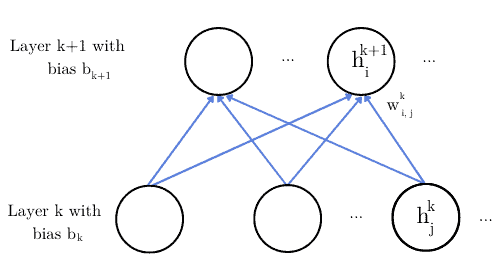
For the general case, Equation (6) becomes:
(15) 
Following the same approach, we can derive the general formula for the partial derivative of the bias units:
(16) 
 Training
We shouldn’t confuse the backpropagation algorithm with the training algorithms. Backpropagation is a strategy to compute the gradient in a neural network. The method that does the updates is the training algorithm. For example, Gradient Descent, Stochastic Gradient Descent, and Adaptive Moment Estimation.
Lastly, since backpropagation is a general technique for calculating the gradients, we can use it for any function, not just neural networks. Additionally, backpropagation isn’t restricted to feedforward networks. We can apply it to recurrent neural networks as well.
In this article, we explained the difference between Feedforward Neural Networks and Backpropagation. The former term refers to a type of network without feedback connections forming closed loops. The latter is a way of computing the partial derivatives during training.
When using a model after training, the input “flows” forward through the layers from the input to the output. But, while training the network using backpropagation, we update the parameters in the opposite direction: from the output layer to the input one.