

Learn through the super-clean Baeldung Pro experience:
>> Membership and Baeldung Pro.
No ads, dark-mode and 6 months free of IntelliJ Idea Ultimate to start with.
Last updated: February 28, 2025
Learn through the super-clean Baeldung Pro experience:
>> Membership and Baeldung Pro.
No ads, dark-mode and 6 months free of IntelliJ Idea Ultimate to start with.
There is a lot of confusion about the difference between Backpropagation (BP) and Stochastic Gradient Descent (SGD). This is not surprising when you consider that even some Machine Learning (ML) practitioners get it wrong, further adding to the confusion.
In short, this is the difference. SGD updates the parameters of a predictive model to minimize a loss function. It does that by using the gradients of the loss function with respect to the parameters. BP provides one way to calculate those gradients.
In this tutorial, we’ll arrive at this statement from the ground up. We start with SGD and then explain the assistive role of BP. However, to obtain a solid intuition for SGD, it is beneficial to start with its predecessor: Gradient Descent (GD)
GD is an optimization algorithm that minimizes a target function. It does this by iteratively updating the input parameters of the function, using the gradient to guide the updating.
There are two reasons for starting here:
Firstly, the algorithms of SGD and GD are near-identical. Therefore, gaining an intuition for GD will make SGD easy to understand.
Secondly, SGD was developed due to an inherent weakness of GD. Knowing this weakness will clarify the role of SGD in ML.
Consider a target function  , with
  input variables
  .
.
To start optimizing, we’ll need an initial point in this -dimensional space, say  .
.
Next, we’ll need the gradient at this point:
(1)
So how is this gradient used to update the initial point?
To explain, let’s take the first component,  . Remember that gradients are in the direction of increasing input. Therefore, we want to increase
  if
if  and vice versa if
  .
.
Consequently, we want to add the negative gradient to the current value of  . In this way, we encourage the algorithm to converge to the minimum of the target function.
Let’s put this all together:
(2)
As it stands, this equation will not reliably converge to the minima. Let’s understand why with a simple example.
Take  , a simple one-dimensional quadratic. If we start at
  then the next point is:
(3)
After that, we have  ,
,  , and so on.
To avoid this, we include an adjustable positive factor,  . It is called the learning rate or step size.
Let’s put this into Equation 2:
(4)
Now, if is too large, we may still overshoot the minima or even diverge from it. However, if is too small, we may not converge before the assigned maximum number of iterations. Accordingly, there is a lot to consider in learning rate selection.
Although this method works well, it has an inherent weakness: Computing the gradient is too computationally expensive for target functions with many variables.
This is where SGD comes to the rescue!
SGD has many applications. Nevertheless, we’ll focus on the most typical case: When SGD is used to train a predictive model using data drawn from an underlying distribution. To build a solid intuition of SGD and ML in general, it is worthwhile to explain what that means.
Fundamentally, the universe is built up of components interacting with each other in very complex ways. They can be thought of as data-generating processes.
For a given process, the underlying distribution is simply the probabilities of each possible outcome. However, this distribution is virtually always unknown.
Fortunately, since the components of a given process interact, there is some inherent structure to the associated data. The goal of ML is to extract this structure, the features of the data.
Unfortunately, extracting this structure is difficult and is the main reason why ML will remain an active field for a long time.
Let’s make this more concrete with a simple example.
Take the data-generating process of writing digits by hand. The MNIST dataset contains  images of this process, expressed in a
  grid.
grid.
We can train a predictive model (e.g., a neural network) to extract the features hidden in this dataset. SGD is one way of doing this.
However, this dataset is the result of many modifications, such as pixelating and anti-aliasing the images. Combined with having only a finite sample, the data naturally reflects a noisy representation of the underlying distribution.
The take-home message is this: Predictive models are trained using data drawn from an underlying distribution. Though algorithms like SGD are effective, they are fundamentally limited by the quality of the dataset used to train the model.
With that in mind, let’s dive into the algorithm.
Suppose we have a dataset of samples taken from an underlying distribution,  .
.
We also have a predictive model,  , where
  represents the
  parameters of the model:
  .
.
The dataset is fed into this model to produce outputs:  . Let’s use these outputs to tune the parameters of the model.
To do that, we need to decide on the desired output. Though it is not typically the case, let’s assume this is done for the entire dataset. Now we have our desired outputs,  .
.
Finally, we need to decide how to quantify the difference between the desired and model outputs. We’ll use a cost function, which we’ll aim to minimize.
The type of model prediction will inform which cost function is most appropriate. For example, a sensible choice for regression problems is the Mean Square Error:
(5)
We could use GD to compute the gradient of the cost function. However, if we assume a large number of parameters and data samples  , that is not computationally feasible.
What separates SGD from GD is that, in each update step, only one sample is fed into the cost function rather than the entire dataset.
This is the reason for the term stochastic in SGD, as it provides a noisy estimate for the gradient of the entire dataset.
Putting this all together, we have:
(6)
where  is the learning rate, as in Equation 4.
To see where BP fits into this picture, let’s assume that our model is a neural network with multiple layers, with the parameters being the weights of the connections between units.
Consider a connection  from the input data to the first layer. It will modify part of the input, which is further modified in all subsequent layers. Hence, changing the value of will have a non-linear effect on the output of each subsequent layer.
In mathematical terms, this means the computation of  will require the chain rule to evaluate. Adding the fact that
  , obtaining
  can easily become computationally intractable.
The naïve approach would be to compute the gradient for each weight individually. However, in this case, the number of computations would scale exponentially with the number of layers. Therefore, to make SGD a viable option, a more efficient method is needed.
This is where BP comes into play.
Foremost, it is important to state that BP is only one of many ways of computing the gradient in SGD.
We’ll omit the details, which are explained elsewhere.
BP leverages dynamical programming to prevent repeating calculations. This is done by computing gradients one layer at a time, starting from the final layer.
For example, the gradient of the penultimate layer will need to consider that of the final layer. Since the latter has already been calculated, it can be repurposed for the former.
In this way, the computations scale linearly with the number of layers. A considerable improvement from the naïve approach.
The figure below compares the difference in time for a single update as an order of magnitude approximation:
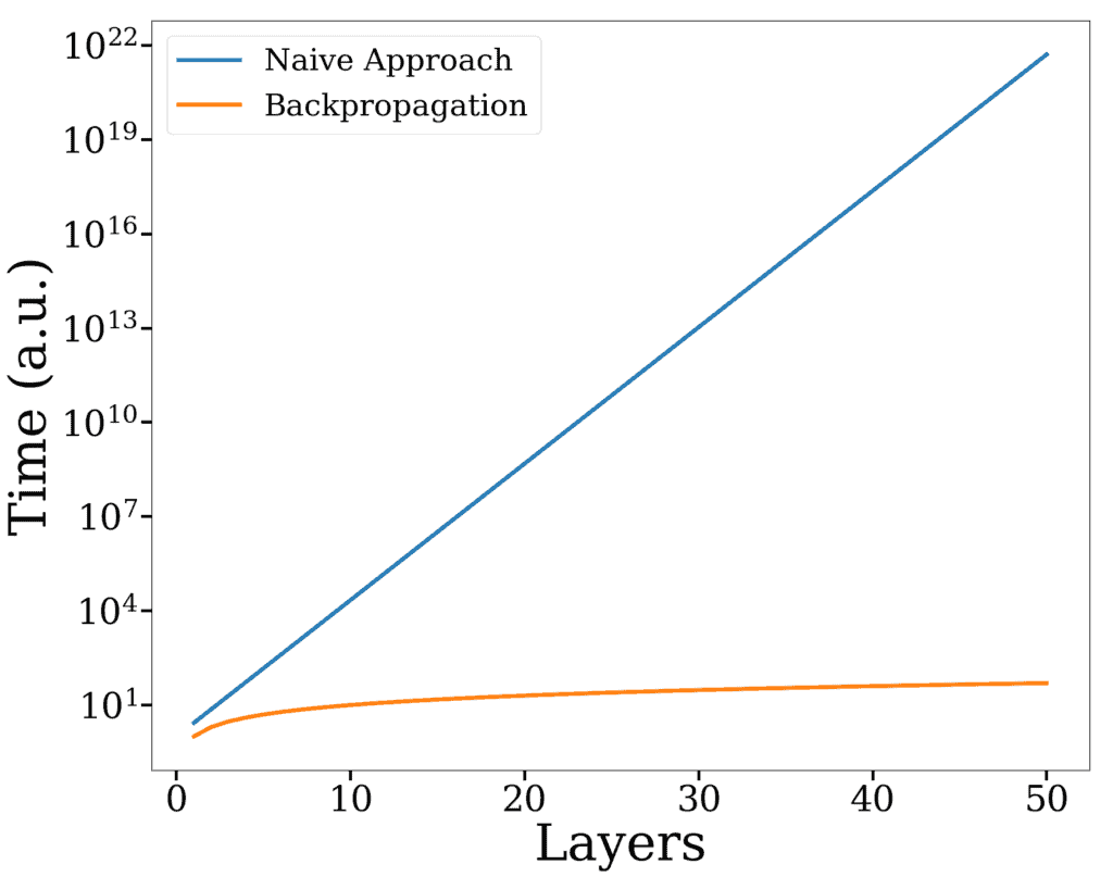
To illustrate numerically, we’ll consider a neural network with 20 layers. In this case, BP will be approximately  million times faster.
Crucially, this speed improvement doesn’t incur a performance cost, as it is just a faster way of computing the same gradient.
To build a strong understanding of SGD, we first explained its precursor, GD. Next, we briefly explored the underlying distribution of a dataset, creating an intuition for the role of SGD in developing predictive models. Finally, we learned that BP is simply a way of efficiently computing the gradients required for SGD.
Hopefully, their respective roles are now clear. However, note that ML practitioners frequently claim to have trained their network using BP. This is technically incorrect and should be interpreted as using SGD with BP to compute the gradients.
![\begin{equation*} \nabla f(\mathbf{a}) = \left[ \frac{ \partial f(\mathbf{a}) }{ \partial a_1}, \frac{ \partial f(\mathbf{a}) }{ \partial a_2}, \cdots, \frac{ \partial f(\mathbf{a}) }{ \partial a_N} \right]. \end{equation*}](/wp-content/ql-cache/quicklatex.com-53bf9cd877c88cad2bcc44af0d51b11d_l3.svg "Rendered by QuickLaTeX.com")


