What Does Learning Rate Warm-up Mean?

1. Introduction

When we’re training neural networks, choosing the learning rate (LR) is a crucial step. This value defines how each pass on the gradient changes the weights in each layer. In this tutorial, we’ll show how different strategies for defining the LR affect the accuracy of a model. We’ll consider the warm-up scenario, which only includes a few initial iterations.

For a more theoretical aspect of it, we refer to another article of ours. Here, we’ll focus on the implementation aspects and performance comparison of different approaches.

2. Setup the Model and Data

To keep things simple, we use the well-known fashion MNIST dataset. Let’s start by loading the required libraries and this computer vision dataset with labels:

import tensorflow as tf
import numpy as np
import matplotlib.pyplot as plt
import keras

fashion_mnist = tf.keras.datasets.fashion_mnist

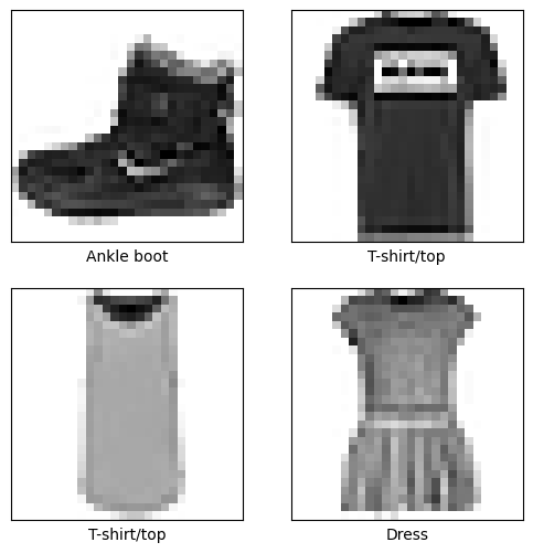
(train_images, train_labels), (test_images, test_labels) = fashion_mnist.load_data()

Let’s take a look at what our data looks like to check if we load everything properly.

class_names = ['T-shirt/top', 'Trouser', 'Pullover', 'Dress', 'Coat', 'Sandal', 'Shirt', 'Sneaker', 'Bag', 'Ankle boot']

# Normalize the data

train_images = train_images / 255.0
test_images = test_images / 255.0

# Plot 4 samples of the dataset

plt.figure(figsize=(6,6))

for i in range(4):
    plt.subplot(2,2,i+1)
    plt.xticks([])
    plt.yticks([])
    plt.grid(False)
    plt.imshow(train_images[i], cmap=plt.cm.binary)
    plt.xlabel(class_names[train_labels[i]])
    
plt.show()

And we can see some samples

We’ll use the same simple architecture for the neural network to keep our comparisons fair.

model = tf.keras.Sequential([
    tf.keras.layers.Flatten(input_shape=(28, 28)),
    tf.keras.layers.Dense(128, activation='relu'),
    tf.keras.layers.Dense(10)
])

Now that we have everything ready, let’s test different LR strategies.

3. LR Strategies

As we said, we’ll evaluate three strategies to define our LR. The first scenario is with a constant value during the warm-up. After that, we propose an LR that increases linearly with the epochs. To conclude, we propose a more robust strategy named Adagrad.

3.1. Constant LR

Given the nature of our problem, we choose a categorical loss function for the model. Then, to use a constant LR equal to $0.01$, we directly define the value when we choose the optimizer:

optimizer = keras.optimizers.Adam(learning_rate=0.01)
model.compile(optimizer=optimizer,
              loss=tf.keras.losses.SparseCategoricalCrossentropy(from_logits=True), metrics=['accuracy'])

Finally, we can fit the model and check the results:

history = model.fit(train_images, train_labels, epochs=5, verbose=1)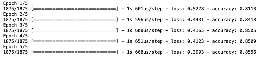

After only $5$ iterations, we already have an accuracy of $0.8556$ and a decreasing loss function. We should remember that our main goal is to investigate how we can implement different LR strategies. We’ll discuss the performance of different methods without discrediting any of them.

3.2. Linear Increase

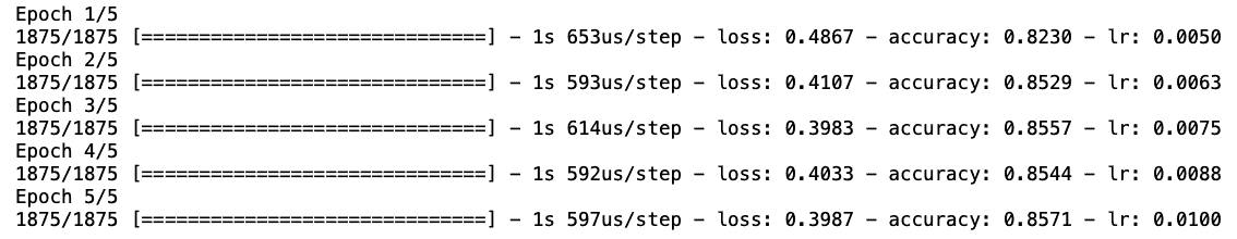
We use the formula defined in the theoretical article for the linear warm-up, mentioned in the introduction. We start with an LR equal to $0.005$ and gradually increase it to $0.01$ in $5$ steps. To pass this strategy to our model, we use the callback API from Keras:

def scheduler(epoch, lr):
    
    initial_lr = 0.005
    final_lr = 0.01
    nsteps = 5
    delta = (final_lr - initial_lr)/(nsteps - 1)
    
    lr = initial_lr + (epoch * delta)
    return (lr)

callback = keras.callbacks.LearningRateScheduler(scheduler)

Then, we fit the model and pass the callback object:

history = model.fit(train_images, train_labels, epochs=5,  callbacks=[callback], verbose=1)
 

As a result, we can see how the LR changes during a linear increase strategy. In the end, we have a satisfactory accuracy ($0.8571$) and LR of $0.01$ for this warm-up. We could now start the training with an LR with the same value to avoid abrupt changes.

3.3. Other Strategies

Besides constant and linear increasing approaches, we can use more complex strategies such as Adagrad or Adadelta. They all have their method of defining the learning rate, leaving us the responsibility of adjusting their parameters.

Let’s start with Adagrad, which is an optimization algorithm that customizes learning rates for individual parameters based on their update frequency during training. This algorithm is built into TensorFlow, and we need only to pass the optimizer an argument. We won’t show explicitly the learning rates after each iteration due to TensorFlow’s limitations:

optimizer = tf.keras.optimizers.Adagrad(
    learning_rate=0.001,
    initial_accumulator_value=0.1,
    epsilon=1e-07,
    name='Adagrad' 
)

model.compile(optimizer=optimizer,
              loss=tf.keras.losses.SparseCategoricalCrossentropy(from_logits=True), 
              metrics=['accuracy'])

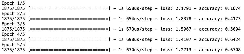
history = model.fit(train_images, train_labels, epochs=5,   verbose=1)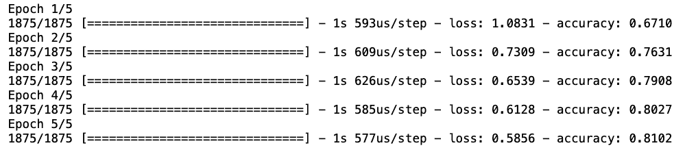

In brief, we can see that we started with a lower initial accuracy that was quickly fixed. This is because Adagrad relies on iterations to learn which parameters are being more frequently updated.

We can also adjust the learning rate for each dimension during training. This is the idea behind Adadelta.In this way, we avoid the problem of accumulating every gradient from previous iterations. To implement, we just need to change the optimizer:

optimizer = keras.optimizers.Adadelta(
    learning_rate=0.001,
    rho=0.95,
    epsilon=1e-07
)

Once again, we started from a very low accuracy that increased significantly after the second epoch.

4. Conclusion

In this article, we discussed implementing different LR strategies to warm up the training stage. This is an important step when training a model, especially if we aim to find a local optimum. Our code and examples enable the optimizer’s choice with few adjustments, serving as a cookbook for prospective tests.