Minimax Algorithm

1. Overview

In the domains of artificial intelligence and game theory, we often come across search problems. Such problems can be described by a graph of interconnected nodes, each representing a possible state.

An intelligent agent needs to be able to traverse graphs by evaluating each node to reach a “good” (if not optimal) state.

However, there are particular kinds of problems where typical graph search algorithms cannot be applied.

In this tutorial, we’ll discuss such problems and evaluate one of the possible solutions – the Minimax algorithm.

2. Introduction

In this tutorial, we’ll be discussing the minimax algorithm, a rather simplistic approach to dealing with adversarial problems. “Adversarial” refers to multi-agent systems, where each agent chooses their strategy by considering the likely actions of their opponents.

A utility function dictates how “good” a state is for the agent. In a 2-player game, the agent tries to maximize the utility function, while his opponent tries to minimize it. The reasoning behind the algorithm’s name becomes apparent.

3. Example

Let’s consider an example to understand how the algorithm functions. Two players, Max and Min, are playing a game that can be represented by a tree, as shown in the image below:

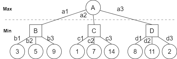
Circles denote that it is Max’s move and squares denote Min’s move. The game ends when a terminal (leaf) node is reached. The terminal value is the utility function’s value written below the leaf node.

In a setting where both Max and Min play optimally, whichever move Max takes, Min will choose the countermove that yields the lowest utility score. Thus, we can decide the best move by following a top-down approach.

We traverse the tree depth-first until we reach the terminal nodes and assign their parent node a value that is best for the player whose turn it is to move.

In this situation, if Max chose , then Min would choose because that’s the lowest possible value. Therefore we assign . If Max chose , then Min would choose and so on:

Having calculated Min’s moves we can proceed to choose the optimal move for Max, which can be expressed as follows:

Therefore, Max will choose , Min will choose and the terminal value for this game will be .

4. Implementation Details

Having understood the basic functionality of the algorithm, let us put it in more formal terms. Minimax, by its nature, is a depth-first search and can be conveniently coded as a recursive function. The procedure is summarized in the following pseudocode:

All nodes of the state tree must be accessed at least once. For a tree of depth with children per node, this amounts to computational complexity.

5. Improvements

As can easily be seen, an algorithm that must access every single node is not very effective. The trees that come up in real-life applications are extremely deep as well as wide. A great example of this is Tic Tac Toe. It’s certainly a simple game, but the state graph associated with it is very complex, having nodes that must be accessed.

While this issue cannot be solved completely, it can be alleviated by discarding subtrees of nodes that are redundant and do not offer better solutions. This process is called Alpha-Beta Pruning.

Let’s review the previous example one more time:

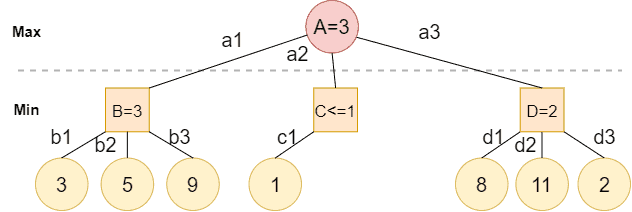
After checking nodes , we know Min will choose because that’s the optimal choice. Therefore node .

When attempting to evaluate node , we notice that the first child node is . Min wants to minimize the utility score, so he will definitely choose unless an even lower value comes up, so we can say that the final value of node will be .

However, node is a better choice for Max since its value is larger than . Therefore we can skip the rest of ‘s children altogether since they won’t offer any better moves. Heading to node , each one of its children will be evaluated because we cannot exclude the chance that a better solution will come up.

We have succeeded in skipping the evaluations of 2 nodes, thereby reducing the computational requirements of the problem. This may not seem like a big achievement, but in more complex applications, the benefits can be pretty significant.

6. Limitations

Although alpha-beta pruning alleviates the computational cost, it only allows the algorithm to check a few layers deeper while remaining within reasonable time constraints. The exponential computational complexity limits the algorithm’s capacity to games with very few layers.

Games with incredibly deep state trees or involve chance tend to be outside the algorithm’s capabilities. In such problems, we need to heuristically evaluate nodes as though they were terminal nodes. This allows the algorithm to examine states at finite depth and choose good but not optimal solutions.

7. Conclusion

In this article, we have discussed the Minimax algorithm’s functionality and the domains where it’s usually applied. Then, we reviewed its weaknesses and introduced a pruning technique that is commonly used to tackle them. Finally, we talked about the limitations of the algorithm and the solutions that form the foundation for more advanced and computationally feasible algorithms.