

Learn through the super-clean Baeldung Pro experience:
>> Membership and Baeldung Pro.
No ads, dark-mode and 6 months free of IntelliJ Idea Ultimate to start with.
Learn through the super-clean Baeldung Pro experience:
>> Membership and Baeldung Pro.
No ads, dark-mode and 6 months free of IntelliJ Idea Ultimate to start with.
In this tutorial, we’ll discuss a random process in mathematics: random walk. We’ll present the definition with examples of different types of random walks.
Finally, we’ll talk about the applications of a random walk.
A random walk can be defined as a series of discrete steps an object takes in some direction. Moreover, we determine the direction and movement of the object in each step probabilistically. In mathematics and probability theory, a random work is a random process.
In a random walk, the future position is entirely independent of the current position of an object. Additionally, it’s an example of the Markov process. Starting from a position, the object can go in any direction. Each step taken by the object in any direction has a probability associated with it. Hence, the final position is completely independent of the point of origin.
A simple example of a random walk is a drunkard’s walk. A drunk man has no preferential direction. Therefore, he’s equally likely to move in all directions.
In the random work concept, the utmost significant problem is finding a probability distribution function that can estimate the probability of the current position of an object after taking a random walk for a fixed amount of time.
The simplest and basic random walk is a one-dimensional walk. Let’s look at a random walk on integers:

So here, an object is standing at point  . It can move in two directions: forwards and backward. Now we’ll decide the direction of each step of the object by flipping a coin. In the case of a head, the object will move forward. If it’s a tail, the object will move backward. Here we’ll flip a coin, move the object one step according to the rule and flip the coin again.
Now let’s start the process. Let’s take the first turn:
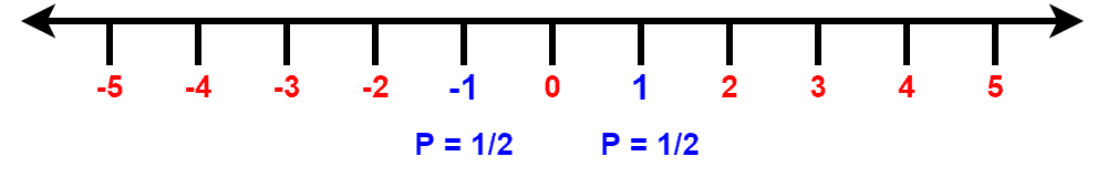
After the first turn, the object can either go to  or
or  position with equal probability
  . Now let’s take the second turn:
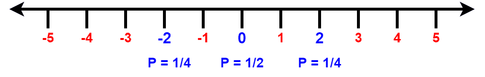
After taking the second step, we can find the object in three positions:  , or
, or  . Here, the probability associated with positions and
  is the same. Although with the probability of , the object might be standing on the position . Likewise, let’s look at the probabilities at the third turn:
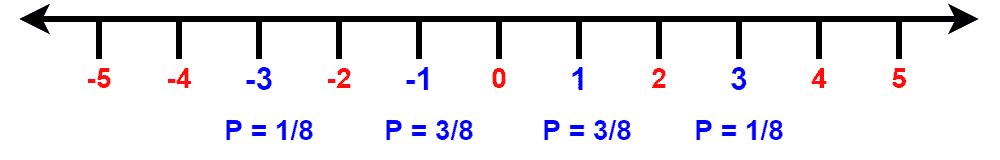
Here the object can be found in  positions. The probability of finding the object in either position
  or
or  is
is  . However, the probability of finding the object in either position
  or is
or is  .
.
Now it’s easy to observe that when the number of turns is odd, all possible positions where the object can go is odd. Similarly, in the case of even turns, all possible positions are even numbers.
Now in order to get more insights from the one-dimensional random walk, let’s assume  indicates the outcome of
  coin in the random process. Hence,
  is the outcome of the first coin flipped at the first turn. Additionally, the variable is known as the random variable.
Now in the case of a one-dimensional random walk, the expected or average value of the random variable  is always
  .
.
A random walk can happen in any dimensional. We’ll discuss the random walk in a two-dimensional integer lattice here. Let’s look at a two-dimensional integer lattice:
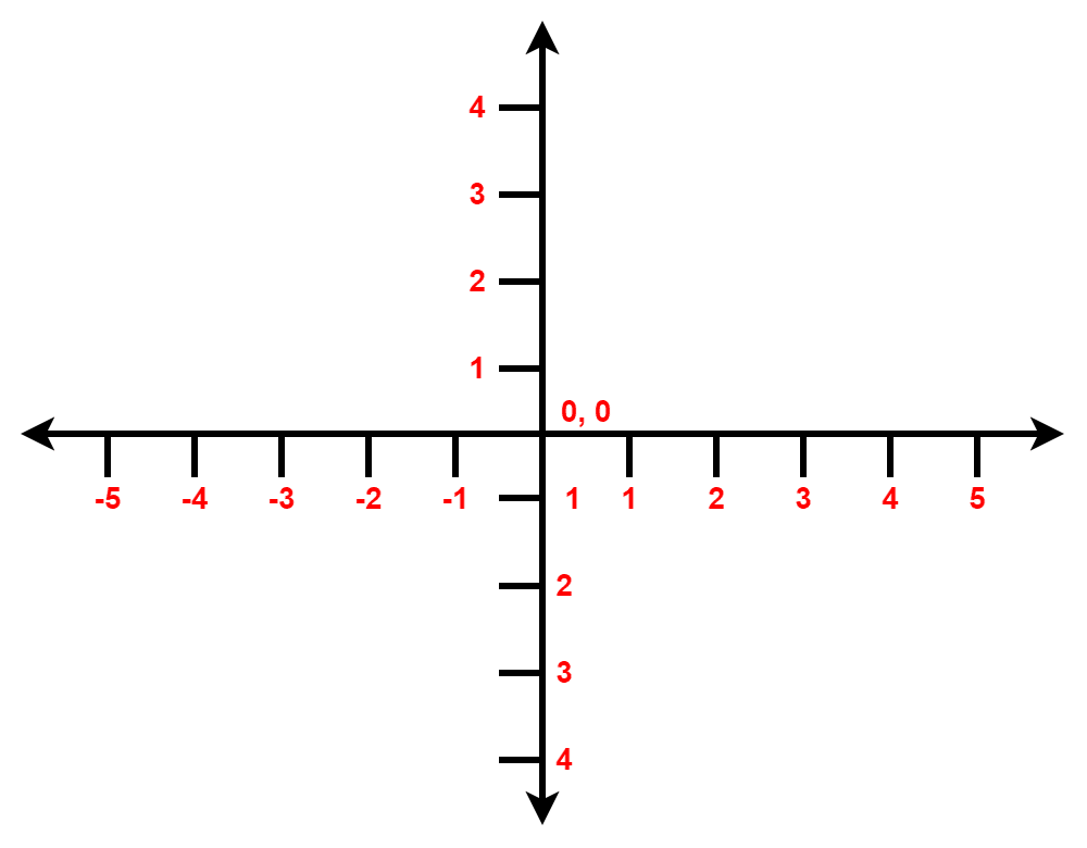
In a two-dimensional random walk, an object can move in four different directions: forward, backward, left, right. Therefore, in this environment, in order to move the object, we need to flip a coin twice at each step. We can decide whether to move the object forward or backward in the first flip. The second flip will determine whether to go in the right or left direction.
Interestingly, in the random walk, the probability of reaching any point in the 2D grid is  when we set the number of steps to infinite.
Let’s now talk about the different types of random walks. There’re two types of random walk based on the position of an object: recurrent and transient.
Recurrent random walks guarantee to return to the starting position starting from a random position. One and two-dimensional random walk falls under this category. We can verify this from the examples presented. Given a large number of steps, it’s guaranteed that the object will return to its starting position.
In contrast to a recurrent random walk, a transient random walk doesn’t guarantee to return to the starting position. In fact, in most cases, there’s a positive probability that the walk will never return to its starting position.
A random walk in 3 or higher dimensions comes under the transient category. The huge number of choices for an object to move at each step makes it impossible to return to the starting position.
There’re many applications of random walk in mathematics, computer science, biology, chemistry, physics. In biological genetic drift, random walks can give us a general idea of the statistical processes involved. In physics, we can use them to describe an ideal chain in polymer physics.
The random work concept is also crucial and used in several fields such as psychology, finance, ecology. Moreover, we can describe fluctuations in the share market with the random walk concept. Additionally, Google search engine algorithms also use them.
In this tutorial, we discuss the concept of random walk in detail. We described random walks in one and two-dimensional with examples.
Finally, we presented various applications of random walk.