

Learn through the super-clean Baeldung Pro experience:
>> Membership and Baeldung Pro.
No ads, dark-mode and 6 months free of IntelliJ Idea Ultimate to start with.
Last updated: March 18, 2024
Learn through the super-clean Baeldung Pro experience:
>> Membership and Baeldung Pro.
No ads, dark-mode and 6 months free of IntelliJ Idea Ultimate to start with.
On the surface, Markov Chains (MCs) and Hidden Markov Models (HMMs) look very similar.
We’ll clarify their differences in two ways: Firstly, by diving into their mathematical details. Secondly, by considering the different problems, each one is used to solve.
Together, this will build a deep understanding of the logic behind the models and their potential applications.
Before doing that, let’s start with their common building block: Stochastic Processes
In short, a stochastic process is a sequence of randomly drawn values that are ordered by an index, such as  .
.
The sequence is stochastic as the elements are drawn from a probability distribution. They are typically used as mathematical models of natural processes and phenomena.
Let’s take the Poisson Point Process as an example:
(1)
where  is the number of occurrences of some event and
  is the expected value of the distribution. The latter is the average number of occurrences we expect before drawing any samples.
This stochastic process is used when the events occur randomly but with an average rate over time. It could be anything from the number of car accidents in a particular area to the number of action potentials a neuron emits.
As a result, each observation has no bearing on the next one. That is, the probability distribution is constant over time. But what if it wasn’t?
That is where MCs come into play.
Consider a discrete system that can be in one of  different states,
  . Each state has a probability of transitioning to the other
  states. This allows us to construct a transition matrix, an
  matrix of transition probabilities.
Let’s say we observe the system for  steps and get the sequence
  , where
  is the state of the system at step
  .
.
What is the probability that the following observation,  , is in state
  , given our observations in the previous steps?
Well, for a stochastic model to be a Markov model, it must only depend on the system’s current state. This is known as the Markov Property.
That means:
(2)
This is true regardless of whether we have an MC or Markov Process. But what is the difference between these two?
Surprisingly, there is not much agreement about what they encompass. Let’s settle on this definition:
A stochastic process with a discrete state space is an MC. However, if the state space is continuous, then it is a Markov Process.
We use a transition kernel instead of a matrix for a Markov Process. Further, we can split both Markov models in discrete or continuous time.
Crucially, if we apply a Markov model to measurements/observations of a physical system, we have to assume the Markov Property. Moreover, since the transition matrix doesn’t change over time, we must assume our physical system is the same.
From there, we have to decide how to model the states of the system. Do we categorize observations into discrete states, or do we allow them to be continuous? We also have to make the same choice for discrete or continuous time.
Using this information, we can proceed in two different ways:
Firstly, let’s say we want to use some observed sequences of states to calibrate our transition matrix. This can be achieved using Maximum Likelihood Estimation (MLE). Put, this asks “what are the parameters of our model that best explains the data we have?”.
Secondly, we can do the opposite: We are sufficiently confident about our choice of transition matrix parameters and want to assess how likely certain sequences are.
Let’s explore these two approaches with a simple example.
We want to predict the number of ants that will be there in the coming days. Suppose we have ants in some box. Every day, we count the number of ants in some small section of the box,  .
.
Let’s assume these states follow the Markov property and that the number of ants in the next day can only increase or decrease by 1.
Therefore, instead of having  parameters, we only have parameters. Also, let’s simplify further and assume these probabilities only depend on the current number of ants in the small section:
(3)
Now, instead of parameters, we have just one:  .
.
To estimate this parameter, we obtain a sequence of the number of ants in the small section. Let’s say we use MLE and obtain  . The figure below shows 20 simulated sequences, starting with 50 ants, with a mean trajectory given in black:
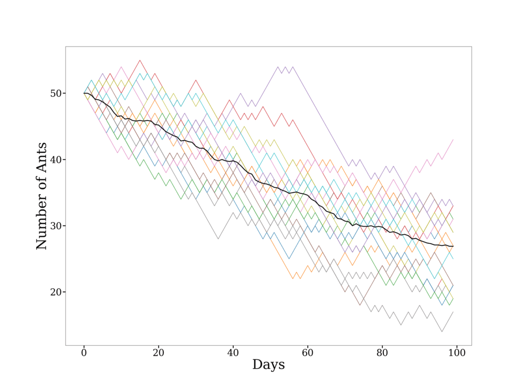
From this, we conclude that the ants seem to be increasingly avoiding that part of the box. This could prompt further investigation as to why this is happening.
Though a silly example, it nicely illustrates the utility of using MCs.
Some systems operate under a probability distribution that is either mathematically difficult or computationally expensive to obtain. In these cases, the distribution must be approximated by sampling from another distribution that is less expensive to sample. Such methods are part of Markov Chain Monte Carlo.
We can observe the states of MCs directly. HMMs are used when we can only observe a secondary sequence. That is, the underlying sequence of states is hidden.
Significantly, this secondary sequence depends on the sequence of hidden states. Therefore, this observed sequence gives us information about the hidden sequence.
Just as the hidden states have a transition matrix, the secondary states have an emission matrix. Each matrix element gives the probability that a given hidden state produces a given observed state.
Since we now have two matrices, the number of parameters can quickly increase with the number of states.
To explain, let’s assume we have  possible observed states and hidden states.
Since the elements of the matrices are probabilities, each row must sum to 1. Therefore, each hidden state has parameters as the last parameter is one minus the sum of the probabilities. In this way, there are parameters to decide on for the transition matrix.
Similarly, each hidden state will “emit” one of different states. These state probabilities must sum to one. So, there are  parameters for the
  emission matrix.
Put together, we have  parameters, which is
  . Even worse, if the states are vectors instead of scalars, then the scaling becomes even more catastrophic!
Although dynamic programming techniques like the Forward Algorithm speed up computations, HMMs are only computationally viable for systems with few hidden states.
Nevertheless, HMMs have a much broader set of applications than MCs.
Broadly speaking, HMMs are a sensible option when the observed sequence of states depends on some unknown underlying factors.
Since MCs do not explicitly consider underlying factors, they are not a good choice here.
Nevertheless, applying HMMs to natural systems is similar to the approach for MCs. The main additional factors are the hidden states.
The applications depend on how much information we have about the model parameters. Let’s briefly outline the two main ones:
Firstly, if we don’t know both the transition and emission matrix elements, we must rely on statistical learning.
In the example for MCs, we used MLE to decide on the best choice for our model parameter. For HMMs, since we have many parameters, we need a more efficient method. The Baum–Welch algorithm is one example.
Secondly, we can perform forecasting if we know the model parameters, as shown in the figure above.
To understand this more intuitively, let’s go back to our simple example.
Let’s say we measured the number of ants in the small section for the 100 days we forecasted. We find that the trajectory did not match our forecast at all.
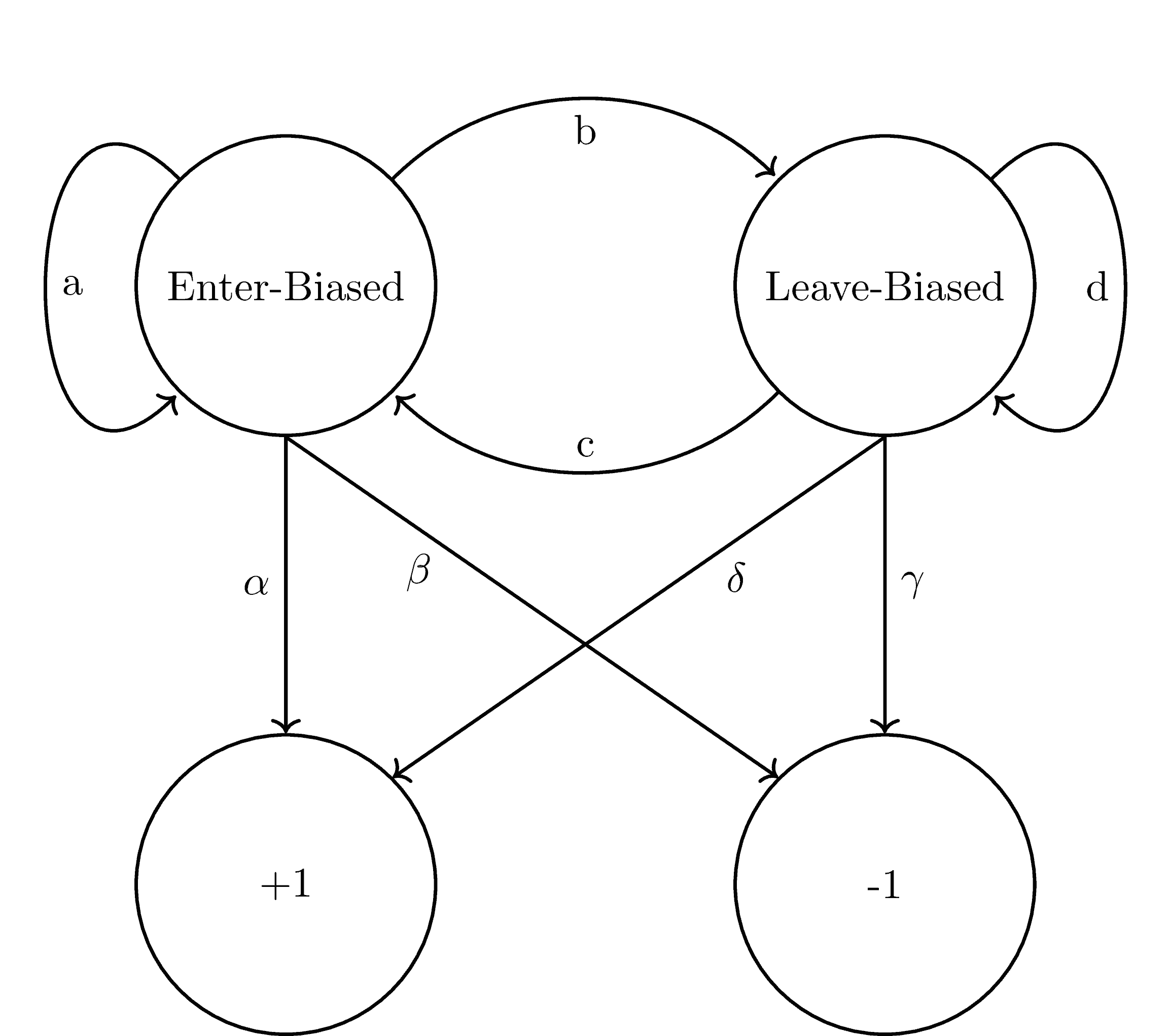
Furthermore, we are informed that the ants exhibit two phases of behavior: One that biases ants to enter the section and another that does the opposite. These are our hidden states.
Instead of looking at the number of ants in the section, we check whether an ant left or arrived. Therefore, we have two observable states,  .
.
Here are our transition  and emission
  matrices:
(4)
In graphical form:
Now, let’s say we collect samples for 100 days and use the Baum-Welch algorithm to determine the parameters that are most likely to explain that data:
(5)
Let’s simulate the trajectories, as we did before, and assume we start in the enter-biased state.
This time, we’ll also add a figure for a single trajectory. It will also include the two states in green and red, for enter-biased and leave-biased, respectively:
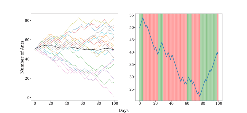
As we can see, the hidden states nicely map onto the ant behavior.
Beyond such forecasting, there are many other analyses to infer the properties of the system.
In this article, we have explained what Stochastic Processes are. MCs and HMMs were outlined and applied to a simple example to clarify their differences using that knowledge.
It is worth stressing that both methods have a vast array of applications and extensions outside this article’s scope.


