Learn through the super-clean Baeldung Pro experience:
>> Membership and Baeldung Pro.
No ads, dark-mode and 6 months free of IntelliJ Idea Ultimate to start with.
Last updated: June 13, 2023

Learn through the super-clean Baeldung Pro experience:
>> Membership and Baeldung Pro.
No ads, dark-mode and 6 months free of IntelliJ Idea Ultimate to start with.
The Mahalanobis distance measures the distance between a point and distribution in  -dimensional space. It’s a very useful tool for finding outliers but can be also used to classify points when data is scarce.
In this tutorial, we’ll learn what makes it so helpful and look into why sometimes it’s preferable to use it over other distance metrics.
Let’s first think about how we can compare just two points  and
and  in an -dimensional space. To measure the overall distance between the two points we’ll need to take into consideration the difference between them on each axis. That is why the formula for -dimensional distance, also called the Euclidean distance, looks like the following:
![\[d(p, q)=\sqrt{\left(p_{1}-q_{1}\right) ^2+\left(p_{2}-q_{2}\right) ^2+\cdots+\left(p_{n}-q_{n}\right)^{2}}\]](/wp-content/ql-cache/quicklatex.com-db328e67b83545e98ade99a8bc6042f4_l3.svg "Rendered by QuickLaTeX.com")
The Euclidean distance is very fundamental and widely used in statistics and machine learning approaches. However, it only makes sense in comparing two points to one another. When we try to compare a point to distribution some caveats need attention.
Usually, to measure the distance between a distribution and a point we would first need to reduce the distribution to a point by finding its mean. After that, we can simply measure the distance to the point in terms of standard deviations from this mean.
This will work in the one-dimensional case but what can we do when there are more dimensions? It might be tempting to use the Euclidean distance as a measure, but when there are multiple variables involved we need to take into account the interconnection between them.
Since the classical Euclidean distance weights each axis equally it effectively assumes that the variables constructing the space are independent and represent unrelated equally important information to one another. If the data we’re working with is like this then using it is entirely fine.
If the variables involved are correlated in some way, however, which is almost always the case with real-world data, we have a problem. Let’s consider the two following scatterplots:
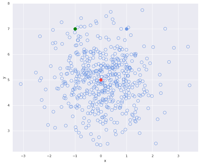
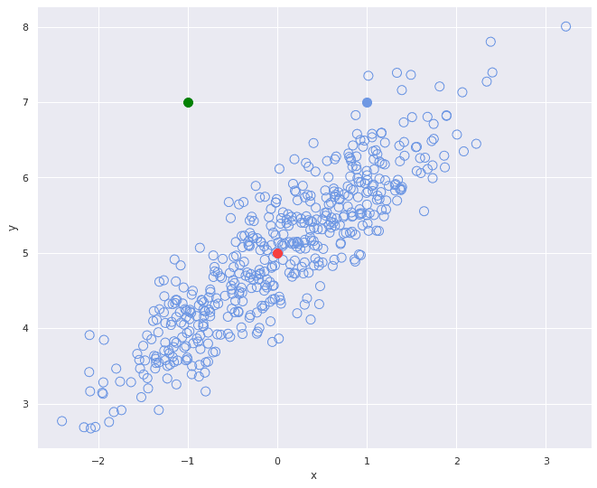
In the first plot, the two variables of the point distribution are uncorrelated, meaning that the  -position of a point doesn’t tell us anything about its
  -position. And on the second graph we can see two positively correlated variables, meaning that as grows, also grows in some amount.
Now let’s turn our attention to the three colored points. If we accept the red point as “the center of mass” of the unfilled points distribution and use it as an anchor we can calculate that the green dot and the blue dot are equally distant from the red center point in Euclidean terms.
Visually however we can see that in the second picture the distance between the green dot and the cluster of unfilled points is somewhat different – in the latter picture the green dot is much more distant from the whole cluster of points.
This is because we’re considering how the whole distribution of unfilled points varies and not focusing on individual points.
Like in our example, correlated variables can give us misleading results if we just use the Euclidean distance straight away. Instead, we can first address the correlation between them. And this is where the Mahalanobis distance comes along. It is defined as:
![\[d_{M}(\vec{p}, \mu ; Q)=\sqrt{(\vec{p}- \mu)^{\top} S^{-1}(\vec{p}- \mu)}\]](/wp-content/ql-cache/quicklatex.com-fbacb27589ae0461c6e5f291dc76d16b_l3.svg "Rendered by QuickLaTeX.com")
where  is the distribution of data points, is the point,
  is the mean vector of , and
  is the inverse of the covariance matrix of all variables.
To better understand the formula, let’s first calculate and compare the actual values taken from the diagram above. The red, green and blue dots are given as follows in both examples:
![\[R = \begin{bmatrix} 0\\ 5\\ \end{bmatrix} \qquad G = \begin{bmatrix} -1\\ 7\\ \end{bmatrix} \qquad B = \begin{bmatrix} 1\\ 7\\ \end{bmatrix}\]](/wp-content/ql-cache/quicklatex.com-94ed75db882732d536946241e5ad45c3_l3.svg "Rendered by QuickLaTeX.com")
The example data was generated using a mean of  and the consequent two covariance matrices:
![\[S_1 = \begin{bmatrix} 1& 0\\0&1 \end{bmatrix} \qquad S_2 = \begin{bmatrix} 1&0.89\\0.89&1 \end{bmatrix} \]](/wp-content/ql-cache/quicklatex.com-04cb90a3d15bc51bdc6a864503d62fa9_l3.svg "Rendered by QuickLaTeX.com")
By the Euclidian distance formula, we can see that the points are equally distant from each other
![\[d(R,G) & = \sqrt {(-1 - 0)^2 + (7 - 5)^2} = \sqrt {5}\]](/wp-content/ql-cache/quicklatex.com-71f5f3938005d915714f266d1a2a5df8_l3.svg "Rendered by QuickLaTeX.com")
![\[d(R,B) & = \sqrt {(1 - 0)^2 + (7 - 5)^2}} = \sqrt {5}\]](/wp-content/ql-cache/quicklatex.com-eb87bc3e986a0d3a5c1c0bbcadcb7170_l3.svg "Rendered by QuickLaTeX.com")
But if we take the distributions into account we get a different result for the green point:
![\[d_{M}(G, \mu ; Q_1)=\sqrt{(\begin{bmatrix} -1\\ 7\\ \end{bmatrix} - \begin{bmatrix} 0\\5\end{bmatrix})^{\top} \begin{bmatrix} 1& 0\\0&1 \end{bmatrix}^{-1}(\begin{bmatrix} -1\\ 7\\ \end{bmatrix} - \begin{bmatrix} 0\\5\end{bmatrix})} = \sqrt {5}\]](/wp-content/ql-cache/quicklatex.com-02def99eaa45c1ac2fee5d3a1c425921_l3.svg "Rendered by QuickLaTeX.com")
![\[d_{M}(G, \mu ; Q_2)=\sqrt{(\begin{bmatrix} -1\\ 7\\ \end{bmatrix} - \begin{bmatrix} 0\\5\end{bmatrix})^{\top} \begin{bmatrix} 1& 0.89\\0.89&1 \end{bmatrix}^{-1}(\begin{bmatrix} -1\\ 7\\ \end{bmatrix} - \begin{bmatrix} 0\\5\end{bmatrix})} \approx 6.416\]](/wp-content/ql-cache/quicklatex.com-b6f583c2d6173a2e0ebdc168f59bb623_l3.svg "Rendered by QuickLaTeX.com")
In the first case where we have zero covariance, we can see that the calculations are equivalent to the Euclidean distance, however, in the second calculation where we have strongly correlated variables, we get a bigger distance for the same point, which matches our initial expectations.
Now, let’s go back to our Mahalanobis distance formula. According to the spectral theorem, we can diagonalize and decompose it into  . And this encapsulates the formula in the more familiar
  :
:
![\[d_{M}(\vec{x}, \vec{y} ; Q)=\|W(\vec{x}-\vec{y})\|\]](/wp-content/ql-cache/quicklatex.com-0a34a7abaef4348a5cd20146bdaa02c4_l3.svg "Rendered by QuickLaTeX.com")
which can be interpreted as the classical Euclidean distance but with some linear transformation beforehand.
In order to understand what kind of transformation is happening it’s useful to turn our attention to the key term – the inverse of the covariance matrix . When multiplying by the inverse of a matrix we’re essentially “dividing”, so in our case, we’re normalizing the variables according to their covariance.
This way the variables are set to have unit variance and look more like the first plot in our illustration. After that, the classical Euclidean distance is applied and we get an unbiased measure of the distance.
In this article, we covered the main arguments for using the Mahalanobis distance instead of classical Euclidean distance when comparing a point to a distribution. We also went over the actual formula that its author made and analyzed why it works.