

Learn through the super-clean Baeldung Pro experience:
>> Membership and Baeldung Pro.
No ads, dark-mode and 6 months free of IntelliJ Idea Ultimate to start with.
Learn through the super-clean Baeldung Pro experience:
>> Membership and Baeldung Pro.
No ads, dark-mode and 6 months free of IntelliJ Idea Ultimate to start with.
In graph theory, there are two main algorithms for calculating the minimum spanning tree (MST):
In this tutorial, we’ll explain both and have a look at differences between them.
Spanning-tree is a set of edges forming a tree and connecting all nodes in a graph. The minimum spanning tree is the spanning tree with the lowest cost (sum of edge weights).
Also, it’s worth noting that since it’s a tree, MST is a term used when talking about undirected connected graphs.
Let’s consider an example:
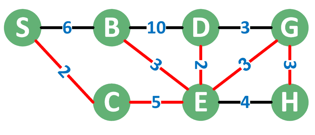
As we can see, red edges form the minimum spanning tree. The total cost of the MST is the sum of the weights of the taken edges. In the given example, the cost of the presented MST is 2 + 5 + 3 + 2 + 3 + 3 = 18.
However, this isn’t the only MST that can be formed. For example, instead of taking the edge between  and
and  , we can take the edge between
  and , and the cost will stay the same. From that, we can notice that different MSTs are the reason for swapping different edges with the same weight.
Therefore, the different order in which the algorithm examines edges with the same cost results in different MSTs. However, of course, all of these MSTs will surely have the same cost.
The main idea behind the Kruskal algorithm is to sort the edges based on their weight. After that, we start taking edges one by one based on the lower weight. In case we take an edge, and it results in forming a cycle, then this edge isn’t included in the MST. Otherwise, the edge is included in the MST.
The problem is with detecting cycles fast enough. In order to do this, we can use a disjoint set data structure. The disjoint set data structure allows us to easily merge two nodes into a single component. Also, it allows us to quickly check if two nodes were merged before.
Therefore, before adding an edge, we first check if both ends of the edge have been merged before. If so, we don’t include the edge in the MST. Otherwise, we add the edge to the MST and merge both nodes together inside the disjoint set data structure.
In this algorithm, we’ll use a data structure named  which is the disjoint set data structure we discussed in section 3.1. Take a look at the pseudocode for Kruskal’s algorithm.
algorithm KruskalAlgorithm:
    // INPUT
    //     edges = the list of all edges in the input graph
    // OUTPUT
    //     Returns the cost and the edges of the minimum spanning tree (MST)

    sort(edges)
    totalCost <- 0
    mst <- []

    for edge in edges:
        // If the current edge does not form a cycle
        if not dsu.isMerged(edge.u, edge.v):
            totalCost <- totalCost + edge.weight
            mst.add(edge)
            dsu.merge(edge.u, edge.v)

    return totalCost, mst
Firstly, we sort the list of edges in ascending order based on their weight. Secondly, we iterate over all the edges. For each edge, we check if its ends were merged before. If so, we just ignore this edge.
Otherwise, we increase the total cost of the MST and add this edge to the resulting MST. Also, we merge both ends of this edge inside the disjoint set data structure.
In the end, we just return the total cost of the calculated MST and the taken edges.
The complexity of the Kruskal algorithm is  , where is the number of edges and
  is the number of vertices inside the graph. The reason for this complexity is due to the sorting cost.
Since the complexity is , the Kruskal algorithm is better used with sparse graphs, where we don’t have lots of edges.
However, since we are examining all edges one by one sorted on ascending order based on their weight, this allows us great control over the resulting MST. Since different MSTs come from different edges with the same cost, in the Kruskal algorithm, all these edges are located one after another when sorted.
Therefore, when two or more edges have the same weight, we have total freedom on how to order them. The order we use affects the resulting MST. Of course, the cost will always be the same regardless of the order of edges with the same weight. However, the edges we add to  might be different.
Another aspect to consider is that the Kruskal algorithm is fairly easy to implement. The only restrictions are having a good disjoint set data structure and a good sort function.
Basically, Prim’s algorithm is a modified version of Dijkstra’s algorithm. First, we choose a node to start from and add all its neighbors to a priority queue.
After that, we perform multiple steps. In each step, we extract the node that we were able to reach using the edge with the lowest weight. Therefore, the priority queue must contain the node and the weight of the edge that got us to reach this node. Also, it must sort the nodes inside it based on the passed weight.
For each extracted node, we add it to the resulting MST and update the total cost of the MST. Also, we add all its neighbors to the queue as well.
In order to obtain a better complexity, we can ensure that each node is presented only once inside the queue. For example, we can use a function  that takes the node with the weight and the edge that led us to this node.
In case the node was already inside the queue, and the new weight is better than the stored one, the function removes the old node and adds the new one instead. Otherwise, if the node isn’t inside the queue, it simply adds it along with the given weight.
Consider the following pseudocode for Prim’s algorithm.
algorithm PrimsAlgorithm:
    // INPUT
    //     G = the given graph
    //     source - the node to start from
    // OUTPUT
    //    Returns the cost of the MST

    totalCost <- 0
    included <- an empty set
    Q.addOrUpdate(source, 0, null)

    while Q is not empty:
        u = Q.getNodeWithLowestWeight()
        totalCost += u.weight

        if u.edge != null:
            mst.add(u.edge)

        included.add(u.node)

        for v in G.neighbors(u.node):
            if v.node not in included:
                Q.addOrUpdate(v.node, weight(u.node, v.node), v.edge)

    return totalCost, mst
In the beginning, we add the source node to the queue with a zero weight and without an edge. We use null to indicate that we store an empty value here. Also, we initialize the total cost with zero and mark all nodes as not yet included inside the MST.
After that, we perform multiple steps. In each step, we extract the node with the lowest weight from the queue. For each extracted node, we increase the cost of the MST by the weight of the extracted edge. Also, in case the edge of the extracted node exists, we add it to the resulting MST.
When we finish handling the extracted node, we iterate over its neighbors. In case the neighbor is not yet included in the resulting MST, we use the function to add this neighbor to the queue. Also, we add the weight of the edge and the edge itself.
The complexity of Prim’s algorithm is  , where is the number of edges and is the number of vertices inside the graph.
The advantage of Prim’s algorithm is its complexity, which is better than Kruskal’s algorithm. Therefore, Prim’s algorithm is helpful when dealing with dense graphs that have lots of edges.
However, Prim’s algorithm doesn’t allow us much control over the chosen edges when multiple edges with the same weight occur. The reason is that only the edges discovered so far are stored inside the queue, rather than all the edges like in Kruskal’s algorithm.
Also, unlike Kruskal’s algorithm, Prim’s algorithm is a little harder to implement.
Let’s highlight some key differences between the two algorithms.
| Kruskal | Prim | |
|---|---|---|
| Multiple MSTs | Offers a good control over the resulting MST |
Controlling the MST might be a little harder |
| Implementation | Easier to implement | Harder to implement |
| Requirements | Disjoint set | Priority queue |
| Time Complexity | |
|
As we can see, the Kruskal algorithm is better to use regarding the easier implementation and the best control over the resulting MST. However, Prim’s algorithm offers better complexity.
In this tutorial, we explained the main two algorithms for calculating the minimum spanning tree of a graph. Firstly, we explained the term MST. Secondly, we presented Kruskal’s and Prim’s algorithms and provided analysis for each one.
Thirdly, we summarized by providing a comparison between both algorithms.