Introduction to Inception Networks

1. Overview

In this tutorial, we’ll learn about Inception Networks. First, we’ll talk about the motivation behind these networks and the origin of their name. Then, we’ll describe in detail the main blocks that constitute the network. Finally, we’ll present two versions of the overall architecture of an Inception Network.

2. Motivation

An Inception Network is a deep neural network that consists of repeating blocks where the output of a block act as an input to the next block. Each block is defined as an Inception block.

The motivation behind the design of these networks lies in two different concepts:

• In order to deal with challenging tasks, a deep neural network should be large, meaning it should consist of many layers and many units per layer, similar to Residual Networks
• The features extracted by neural networks should be multi-scale since people observe the world in a multi-scale aspect. Specifically, the human eye first identifies visual patterns in many scales and then merges this information to form a high-level perception of the world. So, a deep neural network should be able to learn features in multiple scales

Inspired by the above, researchers proposed Inception Networks which are very deep neural networks that learn features in multiple scales.

3. Origin of the Name

The origin of the name ‘Inception Network’ is very interesting since it comes from the famous movie Inception, directed by Christopher Nolan. The movie concerns the idea of dreams embedded into other dreams and turned into the famous internet meme below:

The authors of the network cited the above meme since it acted as an inspiration to them. In the movie, we have dreams within dreams. In an inception network, we have networks within networks.

4. Main Blocks

To gain a better understanding of Inception Networks, let’s dive into and explore its individual components one by one.

4.1. 1 x 1 Convolution

The goal of a convolution is to reduce the dimensions of the input data by channel-wise pooling. In this way, the depth of the network can increase without running the risk of overfitting.

In a 1 1 convolution layer (also referred to as the bottleneck layer), we compute the convolution between each pixel of the image and the filter in the channel dimension. As a result, the output will have the same height and width as the input, but the number of output channels will change.

In the image below, we can see an example of a 1 1 convolution. The input dimension is (64, 64, 192) while the output dimension is (64, 64, 1). So, the dimension of the output feature map is (64, 64, number of filters):

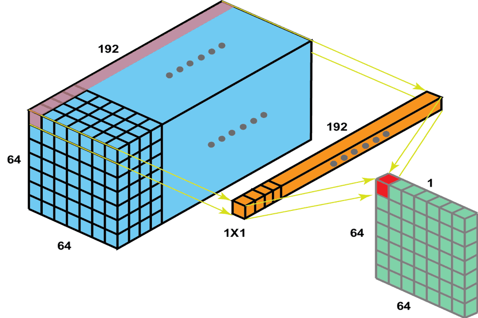
We can also observe that 1 1 convolutions help the network to learn depth features that span across the channels of the image.

4.2. 3 x 3 and 5 x 5 Convolutions

The goal of 3 3 and 5 5 convolutions is to learn spatial features at different scales.

Specifically, by leveraging convolutional filters of different sizes, the network learns spatial patterns at many scales as the human eye does. As we can easily understand, the 3 3 convolution learns features at a small scale while the 5 5 convolution learns features at a larger scale.

5. Overall Architecture

Overall, every inception architecture consists of the above inception blocks that we mentioned, along with a max-pooling layer that is present in every neural network and a concatenation layer that joins the features extracted by the inception blocks.

Now, we’ll describe two Inception architectures starting from a naive one and moving on to the original one, which is an improved version of the first.

5.1. Naive Inception

A naive implementation is to apply every inception block in the input separately and then concatenate the output features in the channel dimension. To do this, we need to ensure that the extracted features have the same width and height dimensions. So, we apply the same padding in every convolution.

Below, we can see an example where the input has dimensions (28, 28, 192) and the output has dimensions (28, 28, channels) where the channels are equal to the sum of the channels extracted from each residual block:

5.2. Optimized Inception

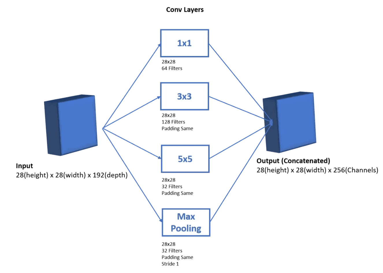
The drawback of the naive implementation is the computational cost due to a large number of parameters in the convolutional layers.

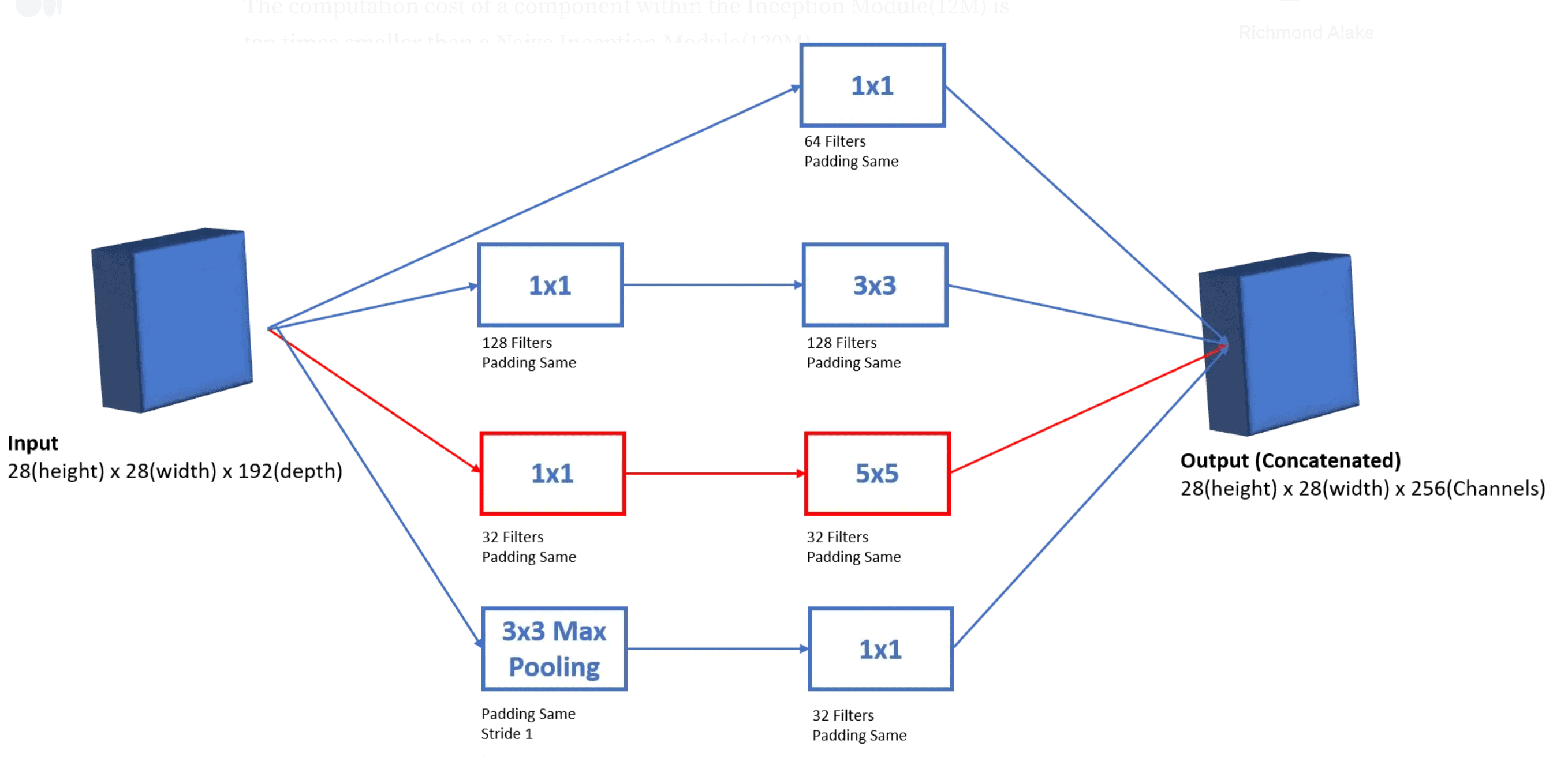
The proposed solution is to take advantage of convolutions that are able to reduce the input dimensions resulting in much lower computational cost.

Below, we can see how the improved inception architecture is defined. We can see that before each 3 3 and 5 5 convolution we add a 1 1 convolution to reduce the size of the features:

6. Conclusion

In this article, we introduced Inception Networks. First, we discussed the motivation behind these networks and the origin of their name. Then, we defined the main inception blocks and presented two versions of inception architectures.