Calculate the Output Size of a Convolutional Layer

1. Overview

In this tutorial, we’ll describe how we can calculate the output size of a convolutional layer. First, we’ll briefly introduce the convolution operator and the convolutional layer. Then, we’ll move on to the general formula for computing the output size and provide a detailed example.

2. Convolution Operation

Generally, convolution is a mathematical operation on two functions where two sources of information are combined to generate an output function. It is used in a wide range of applications, including signal processing, computer vision, physics, and differential equations. While there are many types of convolutions like continuous, circular, and discrete, we’ll focus on the latter since, in a convolutional layer, we deal with discrete data.

In computer vision, convolution is performed between an image $\mathbf{I}$ and a filter $\mathbf{K}$ that is defined as a small matrix. First, the filter passes successively through every pixel of the 2D input image. In each step, we perform an elementwise multiplication between the pixels of the filter and the corresponding pixels of the image. Then, we sum up the results into a single output pixel. After repeating this procedure for every pixel, we end up with a 2D output matrix of features.

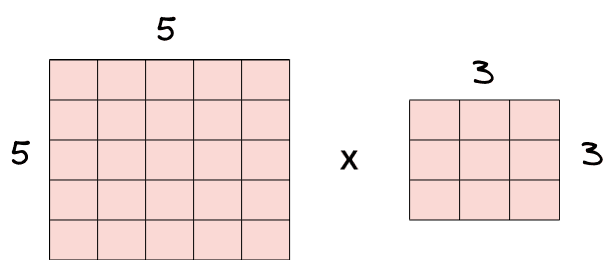
Now let’s describe the above procedure again using a simple example. We have a $5 \times 5$ image $I$ and a $3 \times 3$ filter $K$ that we want to convolve. Below, we can see in bold which pixels of the input image are used in each step of the convolution:

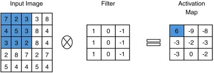
As mentioned earlier, in each step, we multiply the values of the selected pixels (in bold) with the corresponding values of the filter, and we sum the results to a single output. In the example below, we compute the convolution in the central pixel (step=5):

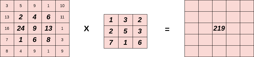
First, we compute the multiplications of each pixel of the filter with the corresponding pixel of the image. Then, we sum all the products:

$2*1+4*3+6*2+24*2+5*9+13*3+1*7+6*1+8*6 = 129$

So, the central pixel of the output activation map is equal to 129. This procedure is followed for every pixel of the input image.

3. Convolutional Layer

The convolutional layer is the core building block of every Convolutional Neural Network. In each layer, we have a set of learnable filters. We convolve the input with each filter during forward propagation, producing an output activation map of that filter. As a result, the network learns activated filters when specific features appear in the input image. Below, we can see an example with the Prewitt operator, a clear filter used for edge detection:

4. Hyperparameters

To formulate a way to compute the output size of a convolutional layer, we should first discuss two critical hyperparameters.

4.1. Stride

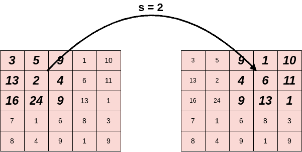
During convolution, the filter slides from left to right and from top to bottom until it passes through the entire input image. We define stride $\mathbf{S}$ as the step of the filter. So, when we want to downsample the input image and end up with a smaller output, we set $S > 0$ .

Below, we can see our previous example when $S = 2$ :

4.2. Padding

In a convolutional layer, we observe that the pixels located on the corners and the edges are used much less than those in the middle. For example, in the below example, we have a $5 \times 5$ input image and a $3 \times 3$ filter:

Below we can see the times that each pixel from the input image is used when applying convolution with $S=1$ :

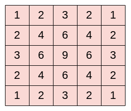
We can see that the pixel $(0, 0)$ is used only once while the central pixel $(3, 3)$ is used nine times. In general, pixels located in the middle are used more often than pixels on edges and corners. Therefore, the information on the borders of images is not preserved as well as the information in the middle.

A simple and powerful solution to this problem is padding, which adds rows and columns of zeros to the input image. If we apply padding $P$ in an input image of size $W \times H$ , the output image has dimensions $(W+2P) \times (H+2P)$ .

Below we can see an example image before and after padding with $P=2$ . As we can see, the dimensions increased from $5 \times 5$ to $9 \times 9$ :

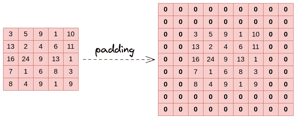
By using padding in a convolutional layer, we increase the contribution of pixels at the corners and the edges to the learning procedure.

5. Formula

Now let’s move on to the main goal of this tutorial which is to present the formula for computing the output size of a convolutional layer. We have the following input:

An image of dimensions $W_{in} \times H_{in}$ .
A filter of dimensions $K \times K$ .
Stride $S$ and padding $P$ .

The output activation map will have the following dimensions:

$\mathbf{W_{out} = \frac{W_{in} - K + 2P}{S} + 1}$
$\mathbf{H_{out} = \frac{H_{in} - K + 2P}{S} + 1}$

If the output dimensions are not integers, it means that we haven’t set the stride $S$ correctly.

We have two exceptional cases:

When there is no padding at all, the output dimensions are $\left(\frac{W_{in} - K}{S} + 1, \frac{H_{in} - K}{S} + 1\right)$ .
In case we want to keep the size of the input unchanged after the convolution layer, we apply same padding where $W_{out} = W_{in}$ and $H_{out} = H_{in}$ . If s=1, we set $p = \frac{K-1}{2}$ .

6. Examples

Finally, we’ll present an example of computing the output size of a convolutional layer. Let’s suppose that we have an input image of size $125 \times 49$ , a filter of size $5 \times 5$ , padding P=2 and stride S=2. Then the output dimensions are the following:

$W_{out} = \frac{125 - 5 + 2*2}{2} = \frac{124}{2} = 62$
$H_{out} = \frac{49 - 5 + 2*2}{2} = \frac{48}{2} = 24$

So,the output activation map will have dimensions $(62, 24)$ .

7. Conclusion

In this tutorial, we talked about computing the outputs size of a convolutional layer.

Full Archive

About Baeldung

Core Concepts

Operating Systems

Artificial Intelligence

Graph Theory

Latex