

Learn through the super-clean Baeldung Pro experience:
>> Membership and Baeldung Pro.
No ads, dark-mode and 6 months free of IntelliJ Idea Ultimate to start with.
Last updated: March 18, 2024
Learn through the super-clean Baeldung Pro experience:
>> Membership and Baeldung Pro.
No ads, dark-mode and 6 months free of IntelliJ Idea Ultimate to start with.
In this tutorial, we’ll learn what is a feature descriptor and why it is an important element in digital image processing. We’ll understand how we can use feature vectors to describe points of interest in an image and how we can use them to identify similar points of interest in different images.
The feature descriptor describes an interest point and encodes the description in the form of a multidimensional feature vector in the vector space.
A point with an expressive texture is an interest point. An interest point is the intersection of two or more edge segments or the point at which the direction of the object’s border rapidly changes.
Interest points are well localized or have a well-defined location in the image space. They maintain their stability when scale, rotation, and light change locally and globally. Therefore, it is crucial that we can compute the interest points accurately, with a high degree of repeatability, and that they should offer effective detection.
A feature descriptor is a method that extracts the feature descriptions for an interest point (or the full image). Feature descriptors serve as a kind of numerical “fingerprint” that we can use to distinguish one feature from another by encoding interesting information into a string of numbers.
A feature is a piece of data that is important for completing the computations necessary for a specific application. Features in an image can be particular elements like points, edges, or objects. A generic neighborhood procedure or feature detection applied to the image may also produce features.
A feature descriptor is the information retrieved from images in the form of numerical values that are challenging for a human to comprehend and correlate. If the image is thought of as data, the features are the details that are drawn from the data.
The dimensions of characteristics extracted from an image are typically substantially smaller than those of the original image. Dimensionality reduction decreases the processing costs associated with image processing.
A mathematical representation of the feature descriptor is a vector with one or more dimensions, called a feature vector. The feature vector is a linear vector that encodes the feature descriptor along a multidimensional feature space, whereas the feature descriptor can be any textual or mathematical-logical description of an interest point.
A feature vector is a vector that includes various informational components about an object. We can create a feature space can by combining object feature vectors. The features could collectively represent a single pixel or an entire image. What we wish to learn or represent about the object decides the level of detail required in the feature vector.
A crucial issue in computer vision is correspondence. The term “correspondence problem” refers to the challenge of determining which elements in one image correlate to which elements in another image when there are changes because of camera movement, the passage of time, or the movement of the objects being photographed.
The correspondence problem is the task of identifying a collection of points in one image that we can recognize with confidence in another image. These images could be the same points in two or more photos of the same 3D scene taken from various angles of view. To do this, we establish corresponding points or corresponding features by matching the points or characteristics in one image with those in the other.
The concept of “vector space” refers to a space made up of vectors, as well as the associative and distributive operations of adding vectors and multiplying vectors by scalars. We can create a feature space by combining object feature vectors.
Any point in an n-dimensional space known as a feature space contains a distinctive feature vector. For instance, a two-dimensional feature space will have two scaler dimensions. Then, we may position any pair of two scalers on this two-dimensional space. After giving each dimension a meaning, we turn this area into a description space for all conceivable concatenations of those meanings.
We know dimensionality as the number of data columns used to represent attributes such as location, color, intensity, neighborhood, and so on. We must choose the dimensions and columns to employ when categorizing or clustering the data to obtain useful information. The number of dimensions in the feature space increases with the level of detail we want to represent.
The feature vector is a point in the n-dimensional feature space. For straightforward situations, consider a two or three-dimensional physical space where one of the feature vectors is a three-dimensional coordinate. However, these vectors may cover hundreds of dimensions in image processing. It could be challenging to picture it as a real spatial location because of this.
To put it simply, a feature vector is a long list of scalers, where each one stands for a different way to describe the object being seen. We can convert a feature vector to an embedding since the characteristics of the feature space are frequently connected. We can transform high-dimensional vectors into an embedding, which is a relatively low-dimensional space.
Using embeddings, we can further simplify machine learning problems when dealing with huge inputs like sparse word vectors. Instead of being a geometric representation of numbers in an n-dimensional space, embeddings are only vectors of numbers.
We must evaluate how closely related two feature vectors are to solve the correspondence problem. This rarely yields a binary outcome but rather a score that indicates how similar one feature vector is to another.
The three most typical comparisons between vectors are the Euclidean distance between the endpoints of the vectors, the cosine of the angle between the vectors, and the dot product, which is the cosine multiplied by the lengths of both vectors. These feature vectors (or embeddings) are sent to a similarity measure, which then calculates a similarity score for them.
It is now possible to compare an interest point from one image to another interest point from a different image to see how similar they are. We specifically set out to address this in the correspondence problem. In image processing and computer vision, similarity metrics and feature vectors are commonly employed.
Depending on the application, we can take two different types of features from the photos. Both local and global elements describe them.
In general, we utilize global features for low-level applications like object detection and categorization, whereas we use local features for higher-level applications like object recognition. While increasing processing overheads, the combination of global and local features enhances recognition accuracy.
Between detection and identification, there is a significant distinction. Detection is finding anything or detecting an object’s presence in the image. Recognition, on the other hand, is determining the identity of the detected object.
Local features represent an image’s texture. A local descriptor describes a patch within an image. Using multiple local descriptors to match an image is more resilient than relying on one sole descriptor. The local descriptors SIFT, SURF, LBP, BRISK, MSER, and FREAK are a few examples.
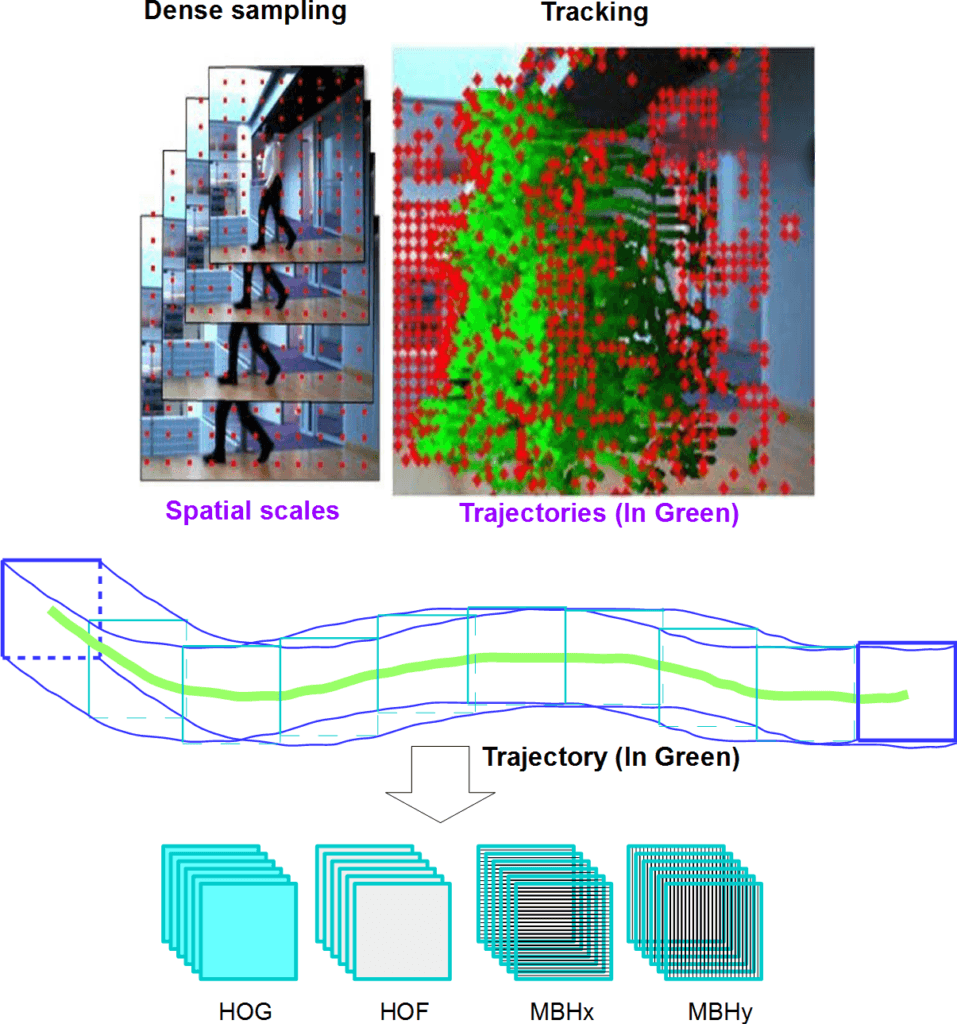
Local features describe the main areas inside an object’s image, whereas global features describe the image as a whole to generalize the complete thing. Contour representations, shape descriptors, and texture features are examples of global features. Global descriptors include things like shape matrices, invariant moments, histogram-oriented gradients (HOG), histograms of optical flow (HOF), and motion boundary histograms (MBH).
The following is an example of sampled interest points and their trajectories (dense trajectories) deploying very long feature vectors by combining HOG, HOF, and MBH feature vectors. We would consider this one of the very advanced use cases of the feature matching workflow discussed in the next section:
The base for the technique used in this example to identify a particular object is identifying point correspondences between the reference and the target images. Despite a scale shift or in-plane rotation, it can still detect objects. It is resistant to little out-of-plane rotation and occlusion as well:
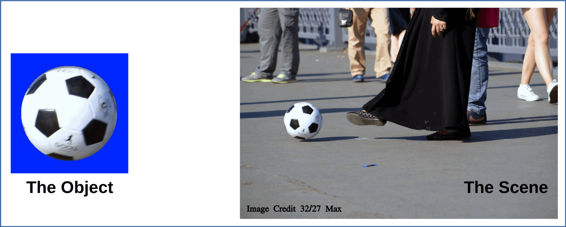
The above pair of images is a feature matching problem statement. The object is a target image that the image processing algorithm wants to locate with confidence in the scene image. No information is available on whether the object is present in the image or not. The only assumption is that there is only one occurrence (if present) of the object in the image. We will now go through the feature matching workflow for the given problem. We will also discuss what happens if the object is not found or when more than one object is found in the image.
The first step in the feature matching workflow is to identify the interest points. Although there could be thousands of interest points in the scene, we often consider only a few hundred top results. This is mainly done to reduce the computational requirements, as only a handful of exact matches are sufficient to locate the object with confidence. Finding the interest points in the two photos:

We now compute the feature vectors for each of the interest points selected for examination. We do this for both the object and the scene images. In both photographs, we pick out the feature descriptors that are of interest:
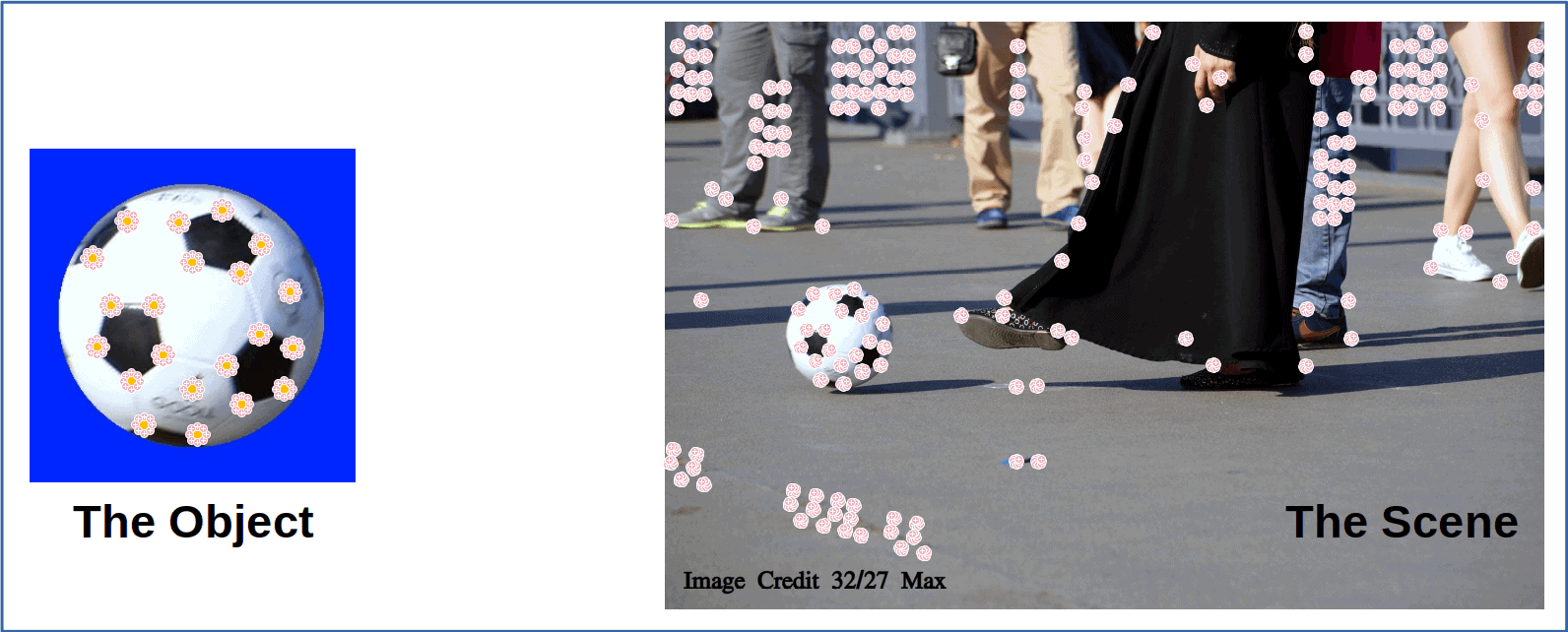
The above figure gives a visual representation of the feature vectors. In reality, each of the feature vectors is a long list of scaler numbers, sometimes spanning hundreds of dimensions.
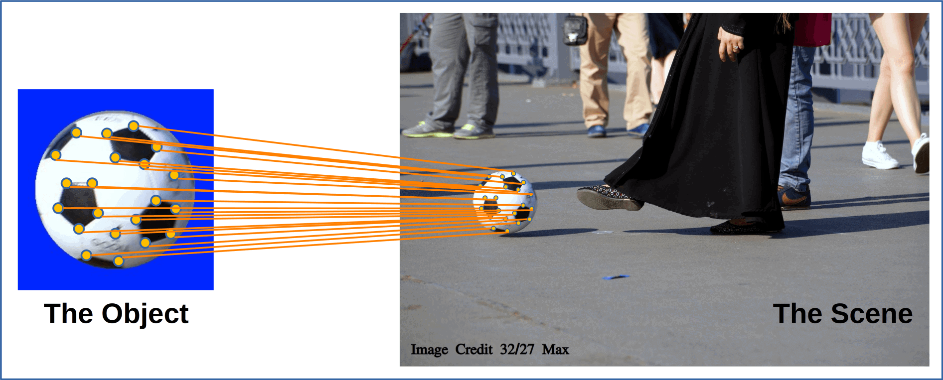
Once we have the feature vectors, the next step is to match them for closeness. This is typically done using one of the similarity measures for feature vectors. One such method includes brute-force matching using Hamming distance. The number of locations at which the matching symbols are different determines the Hamming distance between two strings of equal length.
Another method is brute-force matching using David Lowe’s ratio test. We use this method for the SIFT feature descriptors. Lowe suggested this ratio test to strengthen the SIFT algorithm. This test’s objective is to exclude any spots that aren’t sufficiently distinct. The main principle is that the first-best match and the second-best match should differ sufficiently from one another.
Often, we’re going to need a more advanced parameter drawing technique that allows us to draw only the clear matches using a FLAN-based matcher rather than a Brute-Force matcher. We will utilize a k-dimensional tree, which is an alternate method of data structure organization, to create FLANN parameters. A k-dimensional tree is a space-partitioning data structure used in computer science to organize points in a k-dimensional space.
The results of the matching often include outliers. We can see that most of the matches are correctly pointing to the detected object:
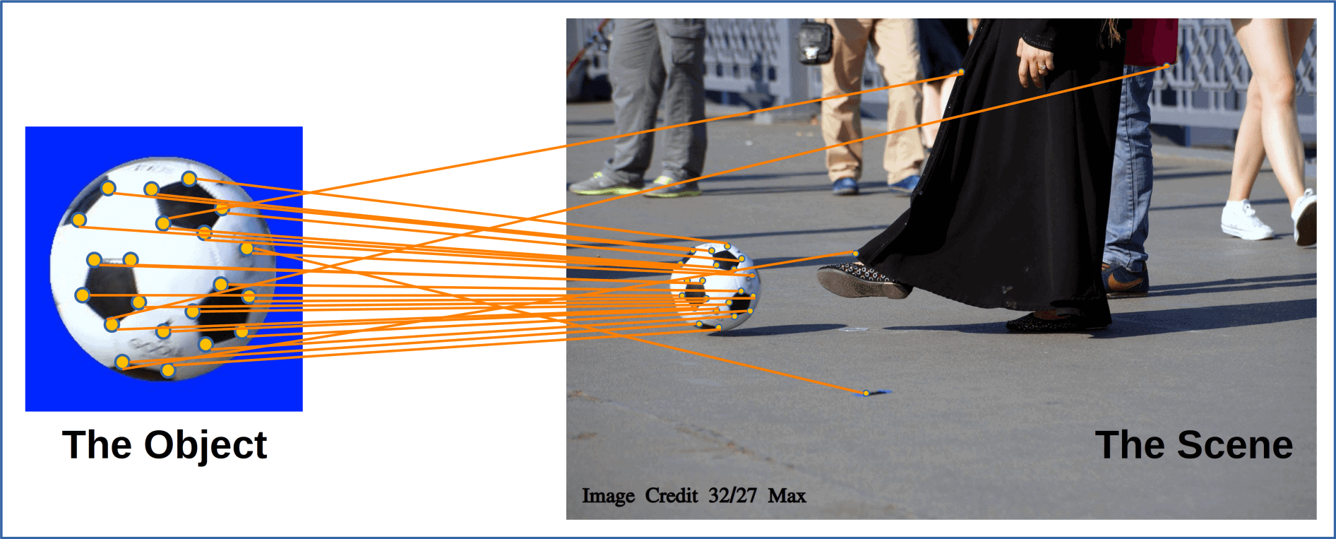
We use geometric information to remove outliers after the feature matching algorithm. Assuming that the object in question is a rigid body with no physical deformations. The scene image contains the object with a different scale and/or rotation. We use this information to remove the outliers. While removing outliers, determine the transformation connecting the matched points. We’re able to localize the object in the scene because of this change:
We often need to mitigate the assumption that there is only one instance of the object in the scene. In such cases, the geometrical transforms for individual matches cluster into more than one group, each of which represents one instance of the detected object. Likewise, we can determine the transformation connecting the matched points for each of these instances.
In case the object is not present in the scene, even one grouping of geometrical transformations won’t exist.
In this article, we learned about feature descriptors, feature vectors, and feature space. We learned how we can use feature vectors to describe points of interest in an image. We learned that the feature matching workflow includes the detection of features, describing them using feature vectors, and then matching them to identify identical points of interest.