

Yes, we're now running our only Summer Sale. All Courses are 30% off until 20th July, 2026:
Learn through the super-clean Baeldung Pro experience:
>> Membership and Baeldung Pro.
No ads, dark-mode and 6 months free of IntelliJ Idea Ultimate to start with.
1. Introduction
In this tutorial, we’ll study the characteristics of one of the simplest and best-known optimization algorithms: hill climbing.
2. Some Definitions
Before approaching the analysis of the algorithm, it is useful to make some definitions that will help us to frame it correctly.
Mathematical optimization problem. It is a problem whose solution involves identifying a maximum or a minimum of some real function, given the values of independent variables or inputs.
Heuristic search. It is a concept counterpoint to deterministic research, which can be used when we have a model that links the quantities to be predicted in the function of the independent variables of the problem or input.
In the absence of a model, a heuristic search may not find the global optimum of the problem, providing a suboptimal solution. However, a constraint is that we achieve the result in a reasonable time (polynomial).
Local search. It’s related to how a heuristic search works. It proposes a certain number of candidates, identifying the one that maximizes some criterion. Local research involves the movement in space of solutions to the problem through the application of local changes. The algorithm ends when we reach the preset stop conditions or when we cannot find further improvements.
Convex optimization. It refers to the type of mathematical functions for which a heuristic method with local research is suitable. They are applied to problems whose objective function (not necessarily continuous in all points) is convex, that is, we have a function such that joining any two points of the function with a segment, it does not lie under the graph of the function.
The following table summarizes these concepts:
| Definition | Description |
|---|---|
| Mathematical optimization | Found maximum o minimum |
| Heuristic search | Mathematical optimization that generates suboptimal solutions |
| Local search | Heuristic search through local changes |
| Convex optimization | Applied to mathematical convex functions |
Hill climbing is a heuristic search method, that adapts to optimization problems, which uses local search to identify the optimum. For convex problems, it is able to reach the global optimum, while for other types of problems it produces, in general, local optimum.
3. The Algorithm
We consider in the continuation, for simplicity, a maximization problem.
For such a problem, hill climbing continuously produces larger values of the target function by making small changes to the current state (local search). If the new state supposes an increase in the value of the objective function it is accepted and becomes the current state of the next step.
Hill climbing is basically a variant of the generate and test algorithm, that we illustrate in the following figure:

The main features of the algorithm are:
- Employ a greedy approach: It means that the movement through the space of solutions always occurs in the sense of maximizing the objective function.
- No backtrackingnderline. It only works in the current state. The past history of the research that led to a certain state is irrelevant.
- Generate and test mechanism. Allows you to decide the next current state.
- Incremental change. The current state is improved through small incremental changes.
4. Limitations of Hill Climbing
Hill climbing is subject to numerous restrictions. To illustrate them, we’ll make use of the so-called state-space diagram, which relates the space of solutions of the problem, which can be reached during the search, with the value of the objective function:

From the figure, it is clear that if the current state corresponds to the one labeled as “local maximum”, a hill climbing algorithm without backtracking is not able to produce further improvements. There are other regions that can lead to convergence problems.
In order to solve the following aberrations, it is necessary to make some changes to the classic hill climbing:
- Allow large jumps, in order to bypass the problem area.
- At each step of the research, study variations in the current state in several directions simultaneously.
- Introduce backtracking, keeping a list of the studied states, tagging those unwanted ones. In this case, we return to one of the states of past history.
- Use a moment term. This adds a correction to the value of the objective function that allows us to penalize problematic or unpromising solutions.
4.1. Plateau or Flat Local Maximum
Points close to the current state have the same value as the objective function. This is a type of local maximum. In this case, the search is hindered because most of the possible motion in the solution space leads to lower objective function values.
4.2. Ridge
It is a region where most of the neighboring points have a value of the objective function lower than that of the current state. At the same time, the figure has a slope, like the one shown in the following figure.
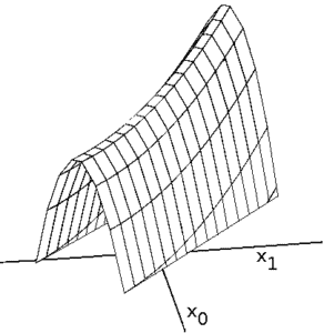
This is a type of local maximum. In this case, the search is hindered because most of the possible motion in the solution space leads to lower objective function values.
4.3. Shoulder
It is a type of plateau in which one of the edges leads to higher objective function values.
The difficulty in this type of aberration is that the algorithm is unable to identify a gradient in the value of the objective function, and therefore can’t choose a direction.
The problem is solved by making a big jump from the current state.
5. Evolution of Classic Hill Climbing
There are two main evolutions of hill climbing, which allow us to completely or partially solve the problems of the previous section. First, let’s talk about the Steepest or Ascent Hill climbing. It examines a set of solutions close to the current state and then selects the best solution from those.
A variant of this technique is the Stochastic Hill Climbing. It selects a single potential solution at random. Based on the extent of the improvement, the algorithm decides whether it will become the new current state or not. This methodology can be declined in different ways, depending on the criterion used in selecting the candidate solution at each step of the calculation.
6. Simulated Annealing
Normally, simulated annealing is not considered a form of hill climbing. In this tutorial, we’ll consider it a particularly advanced evolution of stochastic hill climbing.
The reason for this consideration lies in the fact that both algorithms share the basic mode of operation. In particular, they realize the movement in the space of the states starting from a single solution, the current state. Indeed, the new current state is changed when a solution is found that supposes an improvement to the objective function.
In order to avoid the aberrations of the previous sections, it is necessary to allow the algorithm to “jump” to regions far from the current solution, bypassing problematic areas. This permits extending the application to problems in general. The difference with respect to steepest or stochastic hill climbing is the criterion by which these jumps occur.
6.1. A Physical Analogy to Avoid Entrapment
At the base of simulated annealing, there is a physical analogy: the annealing of a solid. The fraction of particles with given energy depends on the temperature, and they are statistically distributed following the Boltzmann distribution:
![\[n (E) = n_ {0} \exp \left \{- \frac {E} {kT} \right \}\]](/wp-content/ql-cache/quicklatex.com-4557dac54cd5f6f2f3dcd2a6b23ef170_l3.svg "Rendered by QuickLaTeX.com")
where  is the total number of particles and
  is the Boltzmann constant.
6.2. The Metropolis Criterion
The idea of simulated annealing is to allow jumps in the solution space following a similar statistical law. In particular, for a maximization problem:
- We start from an initial state, the current state, with a value of the objective function
 .
. - We define an initial temperature, for example,
 .
. - We generate randomly a new candidate state between already neighboring states. If the objective function of the new state,
 , is greater, then we accept the solution as the new current state, realizing the movement through the solution space.
 - If is less, we accept the solution as the new current state if, generated a random number in the range
![[0: 1]](/wp-content/ql-cache/quicklatex.com-a021366c299d25b14ee1694de00a136d_l3.svg "Rendered by QuickLaTeX.com") , its value is less than the Metropolis criterion:
, its value is less than the Metropolis criterion:
![\[rnd <\exp \left \{- \frac {f_ {0} -f_ {1}} {T} \right \}\]](/wp-content/ql-cache/quicklatex.com-e9e9ee8f7f7d4744c61e26ae93c33346_l3.svg "Rendered by QuickLaTeX.com")
- When a change of state occurs, the temperature decreases. Typically, it follows a law like
 .
. - Execution ends when the temperature reaches a preset value, for example
 .
.
As the temperature drops, acceptance of a new state with a smaller objective function value becomes less likely. This allows the exploration of regions other than the current one with a high probability in the initial phases of the calculation, and with a low probability in the final phases.
Our tutorial The Traveling Salesman Problem in Java covers the implementation in Java of the simulated annealing algorithm.
7. Conclusion
In this tutorial, we took a look at hill climbing. It is a very simple heuristic technique, suitable for certain types of optimization problems such as convex problems. Although simple, it is used in many industrial fields, solving problems in various fields, such as marketing, robotics, and job scheduling problems.
The evolution of hill climbing makes it possible to generalize the application even to problems not within the reach of classic hill climbing. In particular, simulated annealing can also resolve multimodal problems, and in some cases outperforms more advanced algorithms, such as genetic algorithms.