What Is Group Normalization? | Baeldung on Computer Science

1. Introduction

Group Normalization (GN) is a normalization technique used mainly in deep neural networks, mainly in deep learning models such as Convolutional Neural Networks and fully connected neural networks. Yuxin Wu and Kaiming He proposed this technique as an alternative to Batch Normalization.

Normalizing the data is essential to ensure stability during training and facilitate model convergence. Moreover, normalization also helps to reduce sensitivity to hyperparameters and allows for the processing of data with varying scales. All this contributes to a better-performing model and more balanced learning.

In this article, we’ll study GN, its general formula, and how it differs from other normalization approaches.

2. Group Normalization

Group normalization is particularly helpful when dealing with small or variable batches. It works by dividing the channels in a layer into groups and normalizing the resources separately in each group.

In this scenario, a group is simply an independent subset of the channels. Therefore, organize the channels into different groups and calculate the mean and standard deviation along the axes.

The formula commonly used in normalizations is as follows:

$\^{x}_i = \frac{1}{\sigma_i}(x_i - \mu_i)$

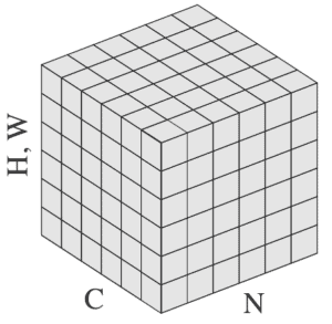
Where $x$ is the feature computed by the layer, and $i$ is the index. In 2D images, represent $i$ by a vector that stores four types of information in the following order (N, C, H, W):

N: represents the group or batch axis;
C: represents the channel axis;
H: spatial height axis;
W: spatial width axis.

To illustrate, the figure below presents these axes in an input tensor:

In addition, $\mu$ and $\sigma$ represent the mean and standard deviation:

$\mu_i = \frac{1}{m} \sum_{k \in S_i} x_k ; \hspace{1cm} \sigma_i = \sqrt{\frac{1}{m} \sum_{k \in S_i} (x_k - \mu_i)^2 + \epsilon}$

In the equation, $\epsilon$ denotes a small constant to avoid division by zero, and $m$ denotes the size of the set. $S_i$ denotes the set of pixels for which the system will calculate the mean and standard deviation.

To sum up, the normalization techniques differ primarily in how they utilize the axes in the calculations. In group normalization, calculate $\mu$ and $\sigma$ along the (H, W) axes and a group of channels.

Therefore, represent a set $S_i$ as follows:

$S_i = \{k | k_N = i_N, \lfloor \frac{k_C}{C/G} \rfloor = \lfloor \frac{i_C}{C/G} \rfloor \}$

In this case, $G$ is the total number of groups. $C/G$ is how many channels are in each group. To simplify things, the channels are grouped in sequential order along the C axis, i.e., $\lfloor \frac{k_C}{C/G} \rfloor = \lfloor \frac{i_C}{C/G} \rfloor$ means that indexes $i$ and $k$ belong to the same group.

During training, GN learns the scale $\gamma$ and shifts $\beta$ parameters per channel just like other normalizations. This is necessary to compensate for any possible loss of representation capacity.

3. Differences Between Group Normalization and Other Approaches

Although the calculation bases for the normalizations are the same, each approach selects the data sets to be normalized differently, making them unique.

If we set $G = 1$ , GN converts to Layer Normalization (LN). For LN, all channels in a layer have similar contributions. However, this is only true in cases of fully connected layers, making it a restricted approach.

If we consider that each group of channels shares the same mean and variance, instead of all channels having the same statistics, GN becomes less restrictive. With this approach, each group can learn a different distribution, increasing the flexibility of the model and resulting in a better representation than the previous technique, LN.

Suppose we consider the opposite scenario, where we define $G = C$ (one channel per group), then GN becomes Instance Normalization (IN). In this case, IN calculates mean and variance only on the spatial dimension, thereby ignoring the relationship between different features. This can restrict effective learning in certain contexts.

Batch normalization calculates the mean and standard deviation along the batch axis to normalize the data. However, when the batch size is small, it can lead to inaccurate estimates of batch statistics. This can increase reported errors as the batch size becomes smaller.

The behavior of GN remains stable across different batch sizes, as its calculation is independent of batch size. This feature of GN enables the model to deliver better results in computer vision tasks, including video classification and object segmentation.

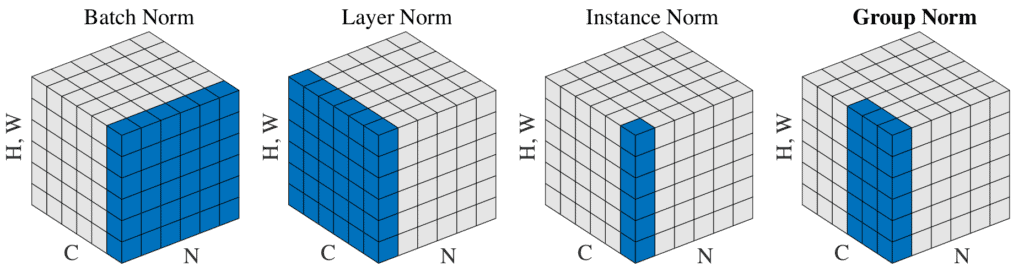
The figure below, taken from page 3 of the original paper, illustrates the difference between the types of normalization. The $S_i$ sets selected for normalization are highlighted in blue. From it, we can see that GN permeates between IN and LN:

Differences Between Group Normalization and Other Approaches

In summary, the choice between normalization approaches depends on the specific context. Each approach has its advantages, and it’s crucial to consider these factors when selecting the most suitable one.

4. Conclusion

In this article, we learned about another normalization approach called Group Normalization.

In conclusion, this approach offers advantages in terms of stability and flexibility. Its batch size-independent nature makes it more robust when applied in scenarios that require online training or mini-batches, for instance.

Full Archive

About Baeldung

Core Concepts

Operating Systems

Artificial Intelligence

Graph Theory

Latex

1. Introduction

2. Group Normalization

3. Differences Between Group Normalization and Other Approaches

4. Conclusion