How to Find Total Number of Minimum Spanning Trees in a Graph?

1. Overview

In this tutorial, we’ll discuss the minimum spanning tree and how to find the total number of minimum spanning trees in a graph.

2. Definition of a Spanning Tree

Let’s start with a formal definition of a spanning tree. Then we’ll define the minimum spanning tree based on that.

For a given graph $\mathbf{G}$ , a spanning tree can be defined as the subset of $\mathbf{G}$ which covers all the vertices of $\mathbf{G}$ with the minimum number of edges.

Let’s simplify this further. Say we have a graph $G$ with the vertex set $V$ , and the edge set $E$ . A spanning tree $T(V_1, E_1)$ on $G$ is a subset of $G$ where $V_1 = V$ and $E_1 \subseteq E$ . So the spanning tree contains all the vertices of the given graph but not all the edges.

Also, we should note that a spanning tree covers all the vertices of a given graph so it can’t be disconnected. By the general property, a spanning tree can’t contain any cycles.

A minimum spanning tree (MST) can be defined on an undirected weighted graph. An MST follows the same definition of a spanning tree. The only catch here is that we need to select the minimum number of edges to cover all the vertices in a given graph in such a way that the total edge weights of the selected edges are at a minimum.

Now, let’s try a graph $G_2$ with $(V_2, E_2)$ . Like a spanning tree, a minimum spanning tree $T_M(V_M, E_M)$ will also contain all the vertices of the graph $G_2$ . Hence, $V_M = V_2$ . The edge set of $T_M$ is the subset of $E_2$ with an objective function: $Minimize$ $\sum_{i=1}^{|E_M|} W[E_M^{i}]$

Here, $|E_M|$ denotes the total number of edges in the minimum spanning tree $T_M$ . The objective function denotes the sum of all the edge weights in $T_M$ , and it should be a minimum among all other spanning trees.

3. Some Examples

In this section, let’s take a graph and construct spanning trees and associated minimum spanning trees to understand the concepts more clearly.

First, let’s take an undirected weighted graph:

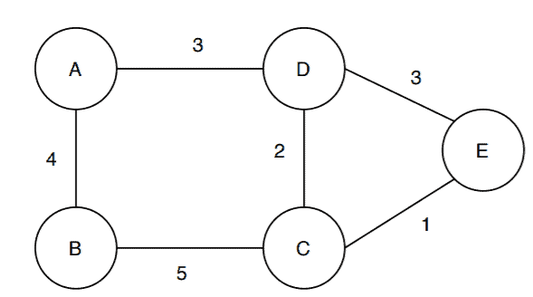
Here, we’ve taken an undirected weighted graph $G_3(V, E, W)$ . Now from the graph $G_3$ , we’ll construct a couple of spanning trees by following the definition of a spanning tree.

Also, we should note that while building the spanning tree, we won’t bother with the edge weights:

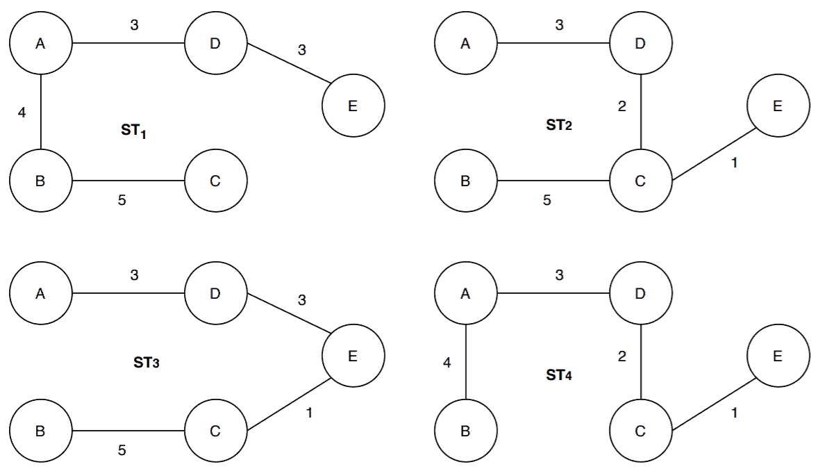
Here we’ve constructed four spanning trees from the graph $G_3$ . Each of the spanning trees covers all the vertices of the graph $G_3$ and none have a cycle.

Now let’s discuss how we can find the minimum spanning tree for the graph $G_3$ . So as per the definition, a minimum spanning tree is a spanning tree with the minimum edge weights among all other spanning trees in the graph.

To find the minimum spanning tree, we need to calculate the sum of edge weights in each of the spanning trees. The sum of edge weights in $ST_1, ST_2, ST_3, ST_4$ are $15, 11, 12,$ and $10$ . Hence, $ST_4$ has the smallest edge weights among the other spanning trees. Therefore, $\mathbf{ST_4}$ is a minimum spanning tree in the graph $\mathbf{G_3}$ .

4. Properties

Let’s list out a couple of properties of a spanning tree. As a minimum spanning tree is also a spanning tree, these properties will also be true for a minimum spanning tree.

In a spanning tree, the number of edges will always be $\mathbf{(|V| - 1)}$ .

For example, let’s have another look at the spanning trees $ST_1, ST_2, ST_3$ , and $ST_4$ . The original graph $G_3$ has $5$ vertices, and each of the spanning trees contains four edges.

A spanning tree doesn’t contain any loops or cycles.

We can see none of the spanning trees $ST_1, ST_2, ST_3,$ and $ST_4$ contain any loops or cycles.

If we remove any one edge from the spanning tree, it will make it disconnected.

Let’s consider the spanning tree $ST_1$ . If we remove any of the edges, it will make it disconnected.

If we add one edge in a spanning tree, then it will create a cycle.

Again we’re considering the spanning tree $ST_1$ . If we add any new edge let’s say the edge $(C, D)$ or $(C, E)$ , it will create a cycle in $ST_1$ .

5. Total Number of MSTs

In this section, we’ll discuss two algorithms to find the total number of minimum spanning trees in a graph.

5.1. When the Graph Is a Complete Graph

If the given graph is complete, then finding the total number of spanning trees is equal to the counting trees with a different label. Using Cayley’s formula, we can solve this problem. According to Cayley’s formula, a graph with $V$ vertices can have $V^{(V-2)}$ different labeled trees.

Therefore, we can say that the total number of spanning trees in a complete graph would be equal to $\mathbf{V^{(V-2)}}$ .

Now to find the minimum spanning tree among all the spanning trees, we need to calculate the total edge weight for each spanning tree. A minimum spanning tree is a spanning tree with the smallest edge weight among all the spanning trees.

Now let’s see the pseudocode:

Here, the variable $N$ denotes the total number of spanning trees in the graph. The variable $P$ is an array that stores the edge list of $N$ spanning trees with their weights. Next, we calculated the sum of edge weights for each $N$ spanning trees and stored it in $minList$ . The minimum value in $minList$ corresponds to the minimum spanning tree.

Finally, we use the variable $countMST$ to denote the total number of minimum spanning trees in the graph.

5.2. When the Graph Is Not Complete

If the given graph is not complete, then we can use the Matrix Tree algorithm to find the total number of minimum spanning trees.

Let’s first see the pseudocode then we’ll discuss the steps in detail:

The first step of the algorithm is to create an adjacency matrix from the given graph. Here $A[m][n]$ denotes an adjacency matrix and $m, n$ is the dimension of the matrix. We should note that in the adjacency matrix, we’ll not consider the edge weights.

The next step is to create a degree matrix from the graph. We can create a degree matrix from the adjacency matrix. We need to replace all the diagonal elements with the degree of the vertices in the graph and all other elements to zero. The variable $D[m][n]$ denotes the degree matrix corresponding to the graph. Again, we’re not considering edge weights here.

Now we calculate the Laplacian matrix by subtracting the adjacency matrix from the degree matrix. The variable $L[m][n]$ represents the Laplacian matrix of the given graph.

To find the total number of spanning trees in the given graph, we need to calculate the cofactor of any elements in the Laplacian matrix. This number is equivalent to the total number of the spanning trees in the graph. The general formula of calculation cofactor in a matrix is: $\mathbf{C_ij = (-1)^{(i+j)}|M_{ij}|}$ , where $i, j$ is the index of the matrix.

In this algorithm, we’ve decided to calculate the cofactor for the value $i=1$ and $j=1$ , which is denoted by the variable $N$ . One can choose any value for $i, j$ .

Next, we store the edge list of each spanning tree with their weights in $P$ . Like the previous algorithm, we calculate the sum of edge weights of each spanning tree denoted by $S$ . Parallelly, we also store the sum of weights in the list $minList$ . The smallest entry in $minList$ is the minimum spanning tree.

To find the total number of minimum spanning trees, we find the occurrence of the smallest entry in $minList$ . The variable $countMST$ gives us the total number of minimum spanning trees in the given graph.

6. Running the Algorithm on a Graph

In this section, we’ll take two graphs: one is a complete graph, and the other one is not a complete graph. For both of the graphs, we’ll run our algorithm and find the number of minimum spanning tree exists in the given graph.

First, let’s take a complete undirected weighted graph:

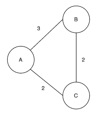
We’ve taken a graph $G_4$ with $3$ vertices. According to our algorithm, the total number of spanning trees in $G_4$ would be: $V^{(V-2)} = 3^{(3-2)} = 3$ . Let’s list out the spanning trees:

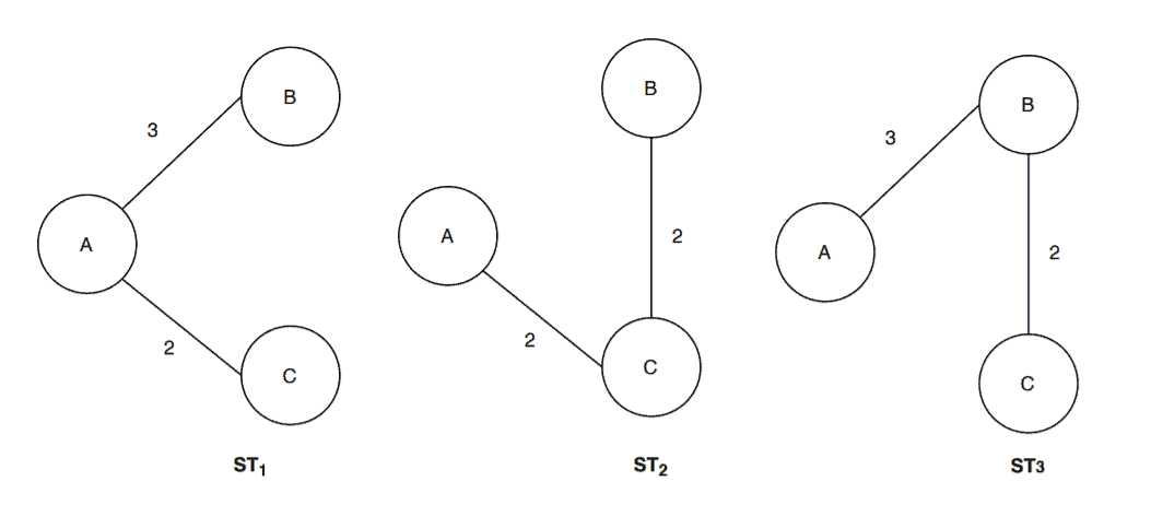
Now to find the minimum spanning tree among the spanning trees, we need to calculate the weights of each spanning tree: $S[ST_1] = 5$ , $S[ST_2] = 4$ , $S[ST_3] = 5$ . We can see that the spanning tree $ST_2$ has the smallest weight among all the spanning trees. Therefore, the number of minimum spanning trees in $G_4$ is $1$ .

Next, let’s take a graph which is not a complete graph:

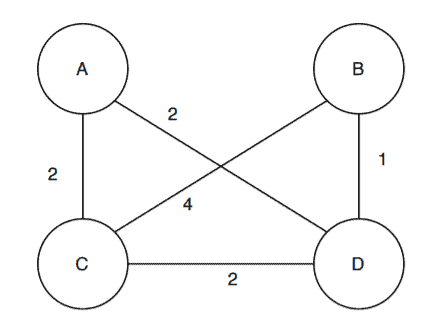
We’re taking a graph $G_5$ here with $4$ vertices. Now the first step is to construct the adjacency matrix of $G_5$ without taking the edge weights:

$\begin{bmatrix} 0 & 0 & 1 & 1\\ 0 & 0 & 1 & 1\\ 1 & 1 & 0 & 1\\ 1 & 1 & 1 & 0 \end{bmatrix} \quad$

Then we’ll construct a degree matrix corresponding to the graph $G_5$ . Again we’ll not consider the edge weights here:

$\begin{bmatrix} 2 & 0 & 0 & 0\\ 0 & 2 & 0 & 0\\ 0 & 0 & 3 & 0\\ 0 & 0 & 0 & 3 \end{bmatrix} \quad$

Next, we’ll create a Laplacian matrix by subtracting the adjacency matrix from the degree matrix:

$\begin{bmatrix} 2 & 0 & 0 & 0\\ 0 & 2 & 0 & 0\\ 0 & 0 & 3 & 0\\ 0 & 0 & 0 & 3 \end{bmatrix} - \begin{bmatrix} 0 & 0 & 1 & 1\\ 0 & 0 & 1 & 1\\ 1 & 1 & 0 & 1\\ 1 & 1 & 1 & 0 \end{bmatrix} = \begin{bmatrix} 2 & 0 & -1 & -1\\ 0 & 2 & -1 & -1\\ -1 & -1 & 3 & -1\\ -1 & -1 & -1 & 3 \end{bmatrix} \quad$

We’re done with the Laplacian matrix. The next step is to calculate any of the positive cofactors from Laplacian matrix. The general formula is : $(-1)^{(i+j)}|M_{ij}|$ . Let’s calculate for $i=1$ and $j=1$ : ${(-1)^{(1+1)}|M_{11}| = (-1)^{2} * ( 2 * ( ( 3 * 3 ) - ( -1 * -1 ) ) ) - ( (-1) * ( ( -1 * 3 ) -( -1 * -1 ) ) )+( (-1) * ( ( -1 * -1 ) - ( -1 * 3 ) ) ) = 8}$

Hence, the number of spanning trees in the graph $G_5$ is $8$ :

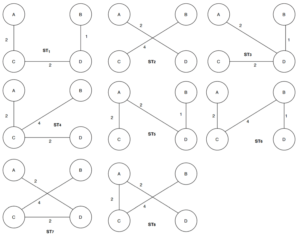
We’re going to calculate the sum of edge weights for each of the spanning tree here. The weights of the spanning trees are: ${S[ST_1] = 5, S[ST_2] = 6, S[ST_3] = 5, S[ST_4] = 8, S[ST_5] = 5, S[ST_6] = 7, S[ST_7] = 8, S[ST_8]= 8}$ .

So clearly, the smallest edge weight among the spinning trees is $8$ . Now in our algorithm, we defined a variable $countMST$ that counts the occurrence of the smallest edge weight in the list $minList$ where all the weights of the spanning trees are stored. We can see the edge weight $5$ occurs three times in the $minList$ , which corresponds to $ST_1, ST_3, and ST_5$ .

Therefore, we applied our algorithm on the graph $\mathbf{G_5}$ and found out that the total number of spanning trees in $\mathbf{G_5}$ is $\mathbf{8}$ and the total number of minimum spanning trees is $\mathbf{3}$ .

7. Time Complexity Analysis

In the case of a complete graph, the time complexity of the algorithm depends on the loop where we’re calculating the sum of the edge weights of each spanning tree. The loop runs for all the vertices in the graph. Hence the time complexity of the algorithm would be $\mathcal{O}\mathbf{(V)}$ .

In case the given graph is not complete, we presented the matrix tree algorithm. Among all the operations, the most expensive one is finding the determining of the matrix. It takes $\mathcal{O}{(V^3)}$ time. Therefore the total time complexity of the algorithm would be $\mathcal{O}\mathbf{(V^3)}$ .

8. Applications of MST

An important application of the minimum spanning tree is to find the paths on the map.

The minimum spanning tree is used to design networks like telecommunication networks, water supply networks, and electrical grids.

Practical applications like cluster analysis, image segmentation, handwriting recognition all use the minimum spanning tree concept.

9. Conclusion

In this tutorial, we’ve discussed how to find the total number of spanning trees and minimum spanning trees in a graph.

We’ve presented two algorithms for two different cases and explained each step in detail. To verify the presented algorithms, we tested it by running the algorithms on two sample graphs.

Full Archive

About Baeldung

Core Concepts

Operating Systems

Artificial Intelligence

Graph Theory

Latex