Finding the Maximum-Minimum Capacity for a Node in a Graph

1. Overview

In this tutorial, we’ll explain the maximum-minimum path capacity problem in graph theory. We’ll define what it is, how to solve it, and how the solution differs from Dijkstra’s.

2. Defining the Problem

The maximum-minimum path capacity problem deals with weighted graphs.

We consider the weight of each edge to represent that edge’s capacity. Our task is to find the path that starts from a source node $source$ and ends at a goal node $goal$ inside the graph. The edge with the lowest capacity in a path forms that path’s capacity.

Among all the paths from $source$ to $goal$ , what we want to do is find the path of maximum capacity.

As a practical example, suppose the graph represents the capacity of water that each pipe can deliver per second. Obviously, we’d be looking for a path that can deliver the largest amount of water per second, and we can’t deliver it any faster than the smallest pipe in the path.

3. Example

Have a look at the following example. We consider the source node to be $S$ and the goal node to be $G$ .

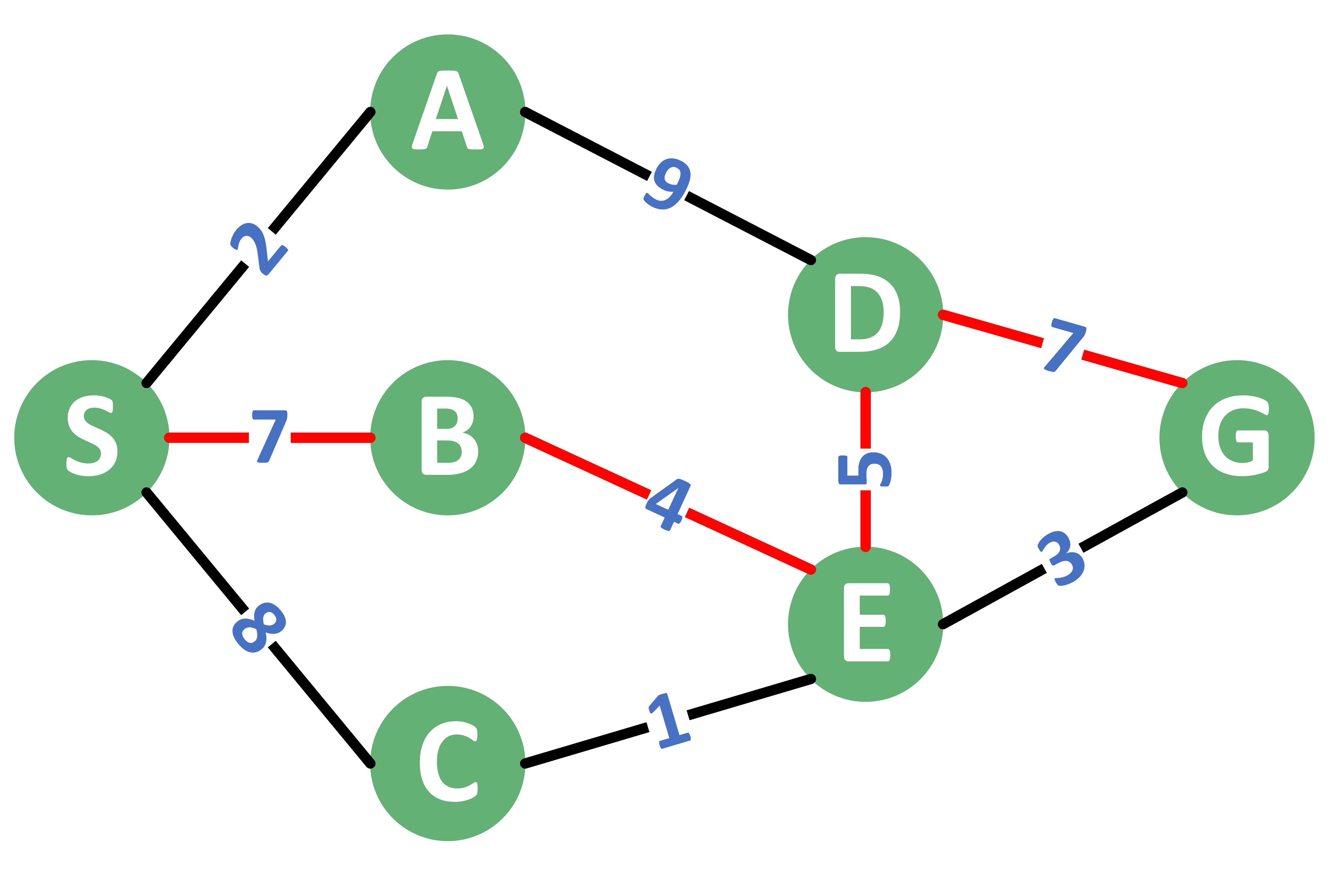
From the graph example, we see that there are multiple paths connecting node $S$ with $G$ . The following table lists the different paths along with their capacity.

Out of all the paths, path number 3 has the largest capacity, which is 4. Therefore, the maximum-minimum capacity for the given graph equals 4.

4. Algorithm

In order to solve this problem, we’ll use a modified version of Dijkstra’s algorithm.

4.1. Differences From Dijkstra’s Algorithm

The pseudocode of this problem is mostly derived from Dijkstra’s algorithm with the following changes:

Instead of having a distance array, we’ll have an array called $capacity$ . This array will store the maximum capacity of each $node$ . By the maximum capacity of a node, we mean the maximum-minimum capacity for all the paths from $source$ to this node.
In Dijkstra’s algorithm, we initialize each node’s distance with .
- For the slot for $source$ , we still do this, indicating that the source node has an unlimited capacity to itself.
- However, for the remaining slots, we’ll initialize the $capacity$ array with $-\infty$ , corresponding to the worst case.
In this problem, when visiting the neighbors of some node, the concept of updating the capacity of a neighboring node is different from the one in Dijkstra’s algorithm. In our case, we update the capacity of each neighboring node with the maximum value among the previous value, the capacity of the node that got us to this neighboring node, and the capacity of the edge we just crossed. Also, we’ll need to update this neighboring node’s capacity inside the data structure we use.
In each step, rather than choosing the node with the lowest cost, we’ll choose the node with the largest capacity.

The proof of this algorithm’s optimality is that we always process the node with the largest capacity. Hence, when we reach the goal node, all the remaining nodes inside the data structure must have a smaller capacity. Therefore, the found path would be the one with the maximum-minimum capacity.

4.2. Pseudocode

Now, let’s review the algorithm in pseudocode:

algorithm findMaxMin(G, source, prev):
    // INPUT
    //     G = the stored graph
    //     source = the source node to start from
    //     prev = the array to store the predecessor of each node
    // OUTPUT
    //     Returns the maximum minimum capacity starting from node source

    capacity <- -infinity
    prev <- undefined
    capacity[source] <- infinity
    Q <- all nodes in the graph

    while Q is not empty:
        u <- Q.getNodeWithMaxCapacity()
        if capacity[u] = -infinity:
            break

        for v in neighbors(u):
            newCapacity <- min(capacity[u], capacityBetween(u, v))
            if newCapacity > capacity[v]:
                capacity[v] <- newCapacity
                prev[v] <- u
                Q.update(v)

    return capacity

First, we initialize the $capacity$ array with $-\infty$ . We’ll also initialize an array $prev$ which will store, for each node $u$ , the node that gets us to reach node $u$ with the maximum path capacity.

Next, we initialize the capacity of the source node with $\infty$ and add all the nodes to $Q$ . The purpose of $Q$ is to find the node with the maximum capacity so far quickly. Also, $Q$ needs to support updating the capacity of some node through the function $update$ . For this, we can use a set that stores the node with its capacity sorted in descending order based on the capacity.

In each step, we extract the node with the maximum path capacity from $Q$ using the function $getNodeWithMaxCapacity$ . If the extracted node has a capacity equal to $-\infty$ , then all the remaining nodes inside $Q$ can’t be reached from $source$ node. Therefore, we can just stop processing further nodes.

Otherwise, we iterate over all the neighbors of node $u$ . for each neighbor, we calculate the new capacity. The new capacity is the minimum between the capacity of node $u$ and the capacity of the edge between $u$ and $v$ . Therefore, we’ve taken the minimum capacity along the path.

After that, we compare the new capacity to the old one for node $v$ . If the new capacity is better, then we update the information of node $v$ with the new capacity. Updating the information of node $v$ includes updating its capacity, updating the $prev$ value for it to become $u$ , and using the function $update$ that removes this node’s object from $Q$ and adds it again with the new path capacity.

Finally, we return $capacity$ , which is the calculated capacity.

The algorithm can be implemented to have a complexity of $O(E \cdot log(V))$ , similar to Dijkstra’s algorithm, where $E$ is the number of edges inside the graph and $V$ is the number of vertices.

4.3. Finding the Path

We’ll use the $prev$ array to restore the path we need. Let’s take a look at the algorithm:

algorithm FindMaxMinPath(G, source, goal):
    // INPUT
    //     G = the stored graph
    //     source = the source node to start from
    //     goal = the goal node to reach
    // OUTPUT
    //     Returns the path with the maximum minimum capacity starting from node source

    findMaxMin(G, source, prev)
    
    u <- goal
    path <- empty list

    while u != undefined:
        path.add(u)
        u <- prev[u]

    reverse(path)
    return path

The algorithm is simple. We start from the $goal$ node. In each step, we add the current node to the path. Also, we move one step back to the previous node using the $prev$ array calculated in $findMaxMin$ function.

Since the $source$ node will have its previous node equal to $undefined$ , we can stop going back once we reach the $undefined$ value.

The complexity of this algorithm (without the findMaxMin function) is $O(V)$ , where $V$ is the total number of vertices inside the graph.

5. Conclusion

In this tutorial, we presented the maximum-minimum capacity in a graph problem. First, we defined the problem. Next, we provided an example that better explains the concept.

After that, we highlighted the main differences between our algorithm and Dijkstra’s algorithm.

Finally, we showed the algorithm.

Full Archive

About Baeldung

Core Concepts

Operating Systems

Artificial Intelligence

Graph Theory

Latex