

Learn through the super-clean Baeldung Pro experience:
>> Membership and Baeldung Pro.
No ads, dark-mode and 6 months free of IntelliJ Idea Ultimate to start with.
Learn through the super-clean Baeldung Pro experience:
>> Membership and Baeldung Pro.
No ads, dark-mode and 6 months free of IntelliJ Idea Ultimate to start with.
Graph Attention Networks (GATs) are neural networks designed to work with graph-structured data. We encounter such data in a variety of real-world applications such as social networks, biological networks, and recommendation systems.
In this tutorial, we’ll delve into the inner workings of GATs and explore the key components that make them so efficient with graphs. We’ll cover the attention mechanism that allows GATs to weigh the importance of each node’s connections, making them particularly adept at handling large and complex graphs.
Graphs are a common data structure in many real-world applications. In a graph, we organize the data into nodes and edges. Nodes represent the entities or objects of interest and edges denote the relationships or connections between the nodes.
We can perform many different machine-learning tasks on graphs.
In a node classification task, our goal is to predict the class or category of each node in a graph. Such a task can be applied, for example, to predict the political affiliation of people in a social network based on their connections to other people.
We can also do link predictions. There, we want to predict which nodes in a graph are likely to be connected in the future. An example is suggesting new products in recommendation systems, based on the users’ buying history and preferences.
Sometimes, we want to classify graphs. Researchers often use this kind of formulation to predict the type of molecule a chemical compound belongs to based on its structural properties.
Finally, there’s the task of community detection, where the goal is to identify groups of nodes that are densely connected and have relatively few connections to nodes outside the group. Solving this kind of problem is very relevant to social networks because it’s important to identify groups of people with similar interests.
Traditional machine learning approaches, such as linear regression and support vector machines, can handle fixed-length vectors of numbers. These methods include mathematical operations that are defined for vectors, such as dot products and Euclidean distances.
On the other hand, we can’t map graphs to vectors easily or sometimes, at all. Graphs consist of nodes and edges, and their numbers in a graph can vary greatly. Additionally, the relationships between nodes in a graph can be highly complex and non-linear, making it difficult to represent them as a simple vector.
Also, graphs can have different types of attributes such as node and edge attributes and also may have different graph structures, each one with its specific meaning, making it harder to apply traditional approaches.
Therefore, researchers have developed specialized machine learning techniques for graph data, such as graph neural networks, or GNNS. GNNs provides a powerful tool for transforming all of the attributes of a graph (nodes, edges, and global context) while preserving symmetries like permutation invariances.
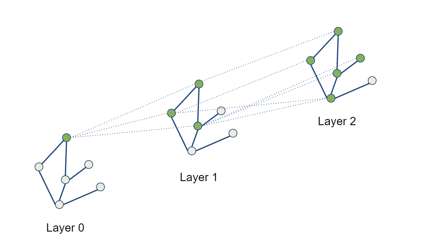
GNNs work by updating the representations of the graph’s nodes through message passing. Each consecutive layer of a GNN updates the current representation of the graph it gets from the previous layer by aggregating the messages received from their immediate neighbors. As such, each message-passing layer increases the receptive field of the GNN by one hop:
Let  be a graph, where
  is its node set and
  represents its edges. Let
  be the neighborhood node
  . Additionally, let
  be the features of node , and
  the features of edge
  .
.
Then, we can express the general form of message passing between nodes:
![\[{\displaystyle \mathbf {h} _{u}=\phi \left(\mathbf {x_{u}},\bigoplus _{v\in N_{u}}\psi (\mathbf {x} _{u},\mathbf {x} _{v},\mathbf {e} _{uv})\right)}\]](/wp-content/ql-cache/quicklatex.com-536826f822e71fd8db7ab9ef18b1723c_l3.svg "Rendered by QuickLaTeX.com")
where  and
and  are differentiable functions (e.g., ReLU), and
  is a permutation invariant aggregation operator that accepts an arbitrary number of inputs (e.g., element-wise sum, mean, or max). Permutation invariance means that we get the same result regardless of the order of inputs. This is important since graphs have no particular node order and each node can have a different number of neighbors.
Additionally, we’ll refer to and as update and message functions, respectively.
The Graph Attention Network architecture also follows this general formulation but uses attention as a form of communication. This mechanism aims to determine which nodes are more important and worth accentuating and which do not add valuable information.
The attention mechanism gives more weight to the relevant and less weight to the less relevant parts. This consequently allows the model to make more accurate predictions by focusing on the most important information.
In the case of GATs, we use the attention mechanism to weigh the importance of the connections between nodes in a graph. Traditional graph convolutional networks (GCNs) use a fixed weighting scheme for the connections, which may not be optimal for all types of graphs. Attention mechanisms, however, allow the model to adaptively assign different weights to different connections depending on the task and the graph structure.
At a high level, GATs consist of multiple attention layers, each of which operates on the output of the previous layer. Each attention layer consists of multiple attention heads, which are separate “sub-networks” operating in parallel.
Inside each attention head, we compute the attention coefficients for a subset of the nodes in the graph. The coefficients represent the relative importance of each node’s connections. We then use these coefficients to weigh the input features of each node. After that, we combine the weighted features and transform them to produce the output of the attention layer.
To do that, we provide the nodes’ features together with the adjacency matrix of the graph, which specifies the connections between the nodes as an input to the attention layer.
We call the main mechanism behind this computation self-attention, which is a type of attention mechanism that allows each node to attend to every other node in the graph, taking into account the connectivity structure of the graph.
Let  be the input features for node
  and
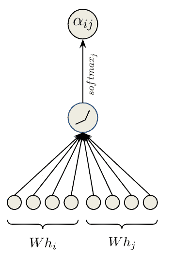
and  a learnable weight matrix. The self-attention mechanism computes the attention coefficients
  for each pair of nodes and
  :
:
![\[\alpha_{ij} = \frac{\exp\left(\text{LeakyReLU}\left(W^T \cdot \left[h_i \Vert h_j\right]\right)\right)}{\sum_{k=1}^{n} \exp\left(\text{LeakyReLU}\left(W^T \cdot \left[h_i \Vert h_j\right]\right)\right)}\]](/wp-content/ql-cache/quicklatex.com-7eb4be4427cfa0b456a902808d156217_l3.svg "Rendered by QuickLaTeX.com")
where  is the concatenation operation and
  is the leaky rectified linear unit activation function:
Once we compute the attention coefficients, we use them to weigh the messages of a node’s neighbors, which are the neighbor’s features multiplied by the same learnable weight matrix . We do this for each attention head and concatenate the result of the heads together:
![\[\displaystyle \mathbf {h} _{u}={\overset {K}{\underset {k=1}{\Big \Vert }}}\sigma \left(\sum _{v\in N_{u}}\alpha _{uv}\mathbf {W} ^{k}\mathbf {x} _{v}\right)\]](/wp-content/ql-cache/quicklatex.com-99f0a0e8d37236d41b27ed3c0ed998ca_l3.svg "Rendered by QuickLaTeX.com")
where  is the number heads and
  is an activation function,
  for example.
We then pass the output to the next attention layer and repeat the process until the final layer. In the final layer, we average the outputs from each attention head before applying the activation function, instead of concatenating. Formally, we can write the final GAT layer as:
![\[\displaystyle \mathbf {h} _{u}=\sigma \left({\frac {1}{K}}\sum _{k=1}^{K}\sum _{v\in N_{u}}\alpha _{uv}\mathbf {W} ^{k}\mathbf {x} _{v}\right)\]](/wp-content/ql-cache/quicklatex.com-7d11cee2ae8dd9ec641c7a41ad28aa18_l3.svg "Rendered by QuickLaTeX.com")
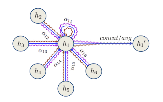
The following diagram provides an overview of the whole aggregation process of a multi-head graph attention layer, where different arrow styles and colors denote independent attention-head computations:
As already mentioned, GATs often can have better predictions when compared to other approaches when applied to tasks such as node classification or link prediction, thanks to the attention mechanism. Nevertheless, GATs can be computationally expensive and require a significant amount of memory to train and evaluate, especially for large graphs.
We calculate the attention weights by applying a linear transformation to the concatenation of the node’s embedding and its neighbor’s embedding, followed by a non-linear activation function. We perform this linear transformation using a set of learnable weight matrices .
The computational complexity of this type of attention mechanism is  , where
  is the number of nodes in the graph, and
  is the dimension of the node embeddings.
For each node, we calculate the attention weight for each of its neighbors by performing a linear transformation on the concatenation of the node’s embedding and the embedding of its neighbor, which results in a total of  linear transformations.
Each linear transformation operation has a computational complexity of  , where is the dimension of the node embeddings.
Therefore, the total computational complexity of this type of attention mechanism is  .
.
It’s worth noting that this is the computational complexity for a single attention head. In practice, GATs often use multi-head attention, which increases the computational complexity by a factor of the number of heads used.
Here’s a quick summary of the advantages and disadvantages of GATs:
| Advantages | Disadvantages |
|---|---|
| The attention mechanism allows the model to focus on specific nodes and edges in the graph. | Can be computationally expensive, especially for large graphs. |
| Can be used to improve performance on tasks such as node classification and graph classification. | The attention mechanisms used may be difficult to interpret. |
| May be sensitive to the choice of hyperparameters, such as the number of attention heads and the number of hidden layers. | |
| May not perform well on graphs with a small number of nodes or edges. |
In this article, we talked about various machine learning tasks that can be performed on graphs and how Graph Neural Networks (GNNs) provide a way to effectively incorporate connectivity information between nodes. Additionally, we covered the basics of GATs and how they work, including the key components of the network and the attention mechanism that allows GATs to weigh the importance of each node’s connections.
Traditional machine learning algorithms work on fixed-length vectors, whereas graph attention networks can handle variable-size graph data.