What Is a Regressor? | Baeldung on Computer Science

1. Overview

In this tutorial, we’ll go over the regressor and use examples to illustrate how to interpret the regressor in different regression models. Furthermore, we’ll go over what the regression analysis is and why we need it.

2. Regressor

A regressor is a statistical term. It refers to any variable in a regression model that is used to predict a response variable. A regressor is also known as:

An independent variable
An explanatory variable
A predictor variable
A feature
A manipulated variable

We use all of these terms depending on the type of field we’re working in: machine learning, statistics, biology, and econometrics.

3. Regression Analysis

Let’s take a look at regression analysis to get a better understanding of the regressor.

A regression analysis allows us to infer or predict a variable on the basis of one or more other variables. Let’s say we want to find out what influences the salary of people:

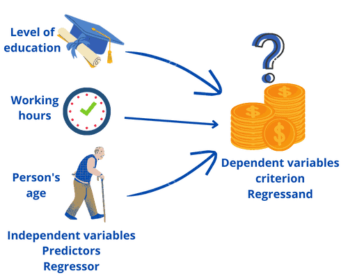
We can predict a person’s salary by taking the highest level of education, the weekly working hours, and the person’s age. The variable that we want to predict is called the dependent variable, regressand, or criterion. The variables we use for the prediction are called regressors, independent variables, or predictors.

Regression analysis can be used to achieve two goals. Let’s take a look at these goals.

3.1. Measurement of the Influence of Variables

So, the first goal is the measurement of the influence of one or more variables on another variable:

Example 1: what influences children’s ability to concentrate
Example 2: do parents’ educational level and place of residence affect children’s future educational attainment

3.2. Prediction of Variables

The second goal is the prediction of a variable by one or more other variables:

Example 1: how long does a patient stay at the hospital
Example 2: what product is a person most likely to buy from an online store

4. Regressor in Regression Models

To construct a regression model, we need to understand how changes in a regressor cause changes in a regressand (or “response variable”).

These models can have one or more regressors. So, the model is referred to as a simple linear regression model when there is only one regressor. When there are multiple regressors, we refer to the model as a multiple linear regression model to indicate that there are multiple regressors.

4.1. Linear Regression With One Regressor

Simple Linear Regression is a linear approach that plots a straight line within data points in order to minimize the error between the line and the data points. It is one of the most fundamental and straightforward types of machine learning regression. So, the relationship between the regressor and regressand is considered to be linear. Let’s take a look at the simple linear regression model:

${Y_{i} = \beta_{0} + \beta_{1}{X_{i}} + \epsilon_{i}}$

where:

${i}$ : the index ${i}$ runs over the observations, ${i= 1, ...., n}$
${Y_{i}}$ : the regressand, or simply the left-hand variable
${X_{i}}$ : the regressor, or simply the right-hand variable
${Y= \beta_{0} + \beta_{1}{X}}$ : the population regression line also called the population regression function
${\beta_{0}}$ : the intercept of the population
${\beta_{1}}$ : the slope of the population
${\epsilon_{i}}$ : the error term

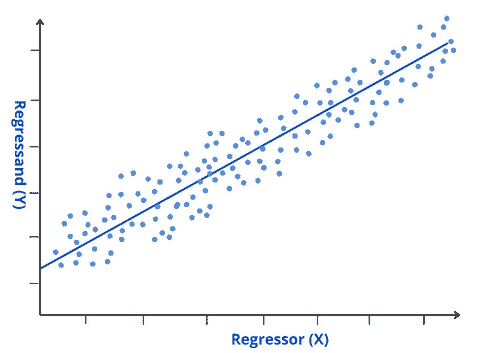
This method is straightforward because it is used to investigate the relationship between one regressor and the regressand. The image below represents how linear regression approximates the relationship between a regressor on the ${X}$ and a regressand on the ${Y}$ axis:

4.2. Example 1: Exam Scores

Let’s take a look at how the number of hours studied affects exam scores. So, we collect data and build a regression model:

${\text{Exam Score} = 68.34 + 3.44 \times (\text{Hours Studied})}$

Let’s see a bloc representation of the model:

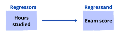
As we can see, our model has only one regressor: $\text{Hours Studied}$ . The coefficient for this regressor indicates that for every additional $\text{Hours Studied}$ , the ${\text{Exam Score}}$ increases by an average of ${3.44}$ points.

4.3. Regression Models With Multiple Regressors

We use the multiple linear regression approach when we have more than one regressor. Polynomial regression is an example of a multiple linear regression approach. So, when multiple regressors are involved, we achieve a better fit than simple linear regression. Let’s take a look at the multiple regression model:

${Y_{i} = \beta_{0} + \beta_{1}{X_{1i}} + \beta_{2}{X_{2i}}+ \beta_{3}{X_{3i}} + .... + \beta_{k}{X_{ki}} + \epsilon_{i}} \text{ , where i = 1, 2, ..., n}}$

where:

${Y_{i}}$ : the ${i^th}$ observation in the regressand. Observations on the ${K}$ regressors are denoted by ${X_{1i}, X_{2i}, ...., X_{ki}}$
The average relationship between ${Y}$ and the regressors is given by the population
${E(Y_{i}|X_{1i} = x_{1}, X_{2i} = x_{2}, X_{3i} = x_{3}, ...., X_{ki} = x_{k}) = \beta_{0} + \beta_{1}{x_{1}} + \beta_{2}{x_{2}}+ \beta_{3}{x_{3}} + .... + \beta_{k}{x_{k}}$
${\beta_{0}}$ : the intercept (it’s the value of ${Y}$ when all ${X}$ s equal ${0}$ )
${\beta_{j} \text{ , where j=1, 2, ..., k}}$ : the coefficients on ${X_{j} \text{ , where j=1, 2, ..., k}}$ . ${\beta_{1}}$ calculates the expected change in ${Y_{i}}$ from a one-unit change in ${X_{1i}}$ while holding all other regressors constant.
${\epsilon_{i}}$ : the error term

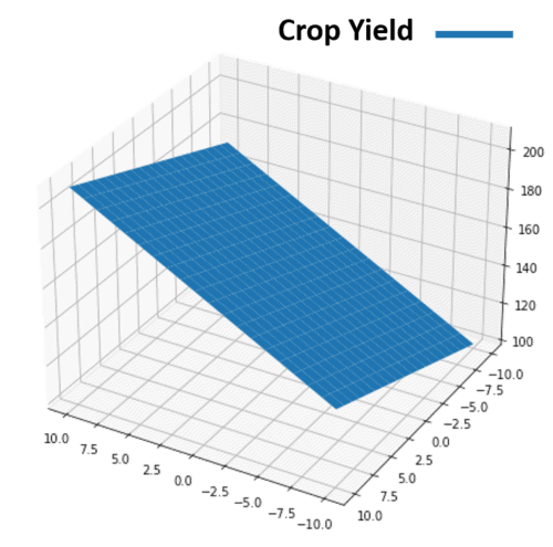
4.4. Example 2: Crop Yield

Let’s take a look at what elements may influence total crop yield (in pounds). So, we collect data and build a regression model:

${\text{Crop Yield} = 154.34 + 3.56 \times (\text{Pounds of Fertilizer}) + 1.89 \times (\text{Pounds of Soil})}$

This model has two regressors: Fertilizer and Soil. Let’s see a bloc representation of the model:

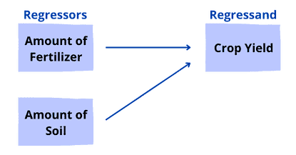
bloc representation with multiple regressor

Let’s interpret these two regressors:

Fertilizer: if the amount of soil remains constant, each additional pound of fertilizer added increases crop output by an average of ${3.56}$ pounds
Soil: if the amount of fertilizer remains constant, each additional pound of soil used increases crop output by an average of ${1.89}$ pounds

The image below represents how multiple linear regression approximates the relationship between regressors ${\text{Fertilizer, Soil}}$ and the regressand ${\text{Crop Yield}}$ :

5. Applications

In machine learning, regression models are trained to understand the relationship between various regressors and a regressand. The model can therefore understand several factors that may lead to the desired regressand.

Let’s take a look at some applications for machine learning regression models:

Forecasting continuous outcomes like sales, stock prices, or house prices
Analyzing datasets to establish the relationships between regressors and regressand
Predicting user trends, such as on e-commerce websites
Predicting future retail sales performance to ensure that resources are used effectively
Creating time series visualizations

6. Conclusion

In this article, we’ve explored the terms regressor and regressand. We’ve also gone over the regression analysis and its types. Then we’ve used examples to unlock their mechanism.

Full Archive

About Baeldung

Core Concepts

Operating Systems

Artificial Intelligence

Graph Theory

Latex