Algorithms to Generate K-Combinations | Baeldung on Computer Science

1. Introduction

In this tutorial, we’ll learn about different algorithms to generate all ${k}$ -element subsets of a set containing ${n}$ elements. This problem is referred to as $k$ -combinations.

The mathematical solution to find the number of $k$ -combinations is straightforward. It’s equal to the binomial coefficient:

$\binom{n}{k} = \frac{n!}{k! (n-k)!}= \frac{n \times (n-1) \times ... \times (n - k + 1)}{k \times (k-1) \times ... \times 1}$

For example, let’s assume we have a set containing 6 elements, and we want to generate 3-element subsets. In this case, there are 6 ways that we can choose the first element. Then, we choose the second element from the remaining 5. Finally, we choose the third and last element of the subset from the remaining 4. The number of choices we’ve had so far is exactly $\frac{n!}{(n-k)!}$ .

Since the ordering of our choices doesn’t matter as we’re constructing a subset, we need to divide by $k!$ . Hence we reach the same formula: $\frac{n!}{k! (n-k)!}$

However, generating all such subsets and enumerating them is more complicated than merely counting them. Let’s have a look at different algorithms that create the subsets in different ways in the following sections.

The algorithms we’ll review in the following sections were initially compiled in “The Art of Computer Programming” by computer scientist Donald Knuth.

2. Lexicographic Generation

Lexicographic order is an intuitive and convenient way to generate $\textbf{k}$ -combinations.

The algorithm assumes that we have a set $S$ containing $n$ elements: {0, 1, … , $n-1$ }. Then, we generate the subsets containing $k$ elements in the form $c_k,c_k-1, ... , c_1$ , starting from the smallest lexicographic order:

The algorithm visits all $k$ -combinations. It recursively represents multiple nested for loops. For example, when $k$ =3, it’s equivalent to 3 nested for loops to generate combinations of length 3:

algorithm visitCombinations(n):
    // INPUT
    //    n = The upper limit for generating combinations
    // OUTPUT
    //    Visits all unique combinations of three different numbers
    //    that are not higher than n.
    
    for c3 in 2 to n - 1:
        for c2 in 1 to c3 - 1:
            for c1 in 0 to c2 - 1:
                // Visit the combination c3, c2, c1
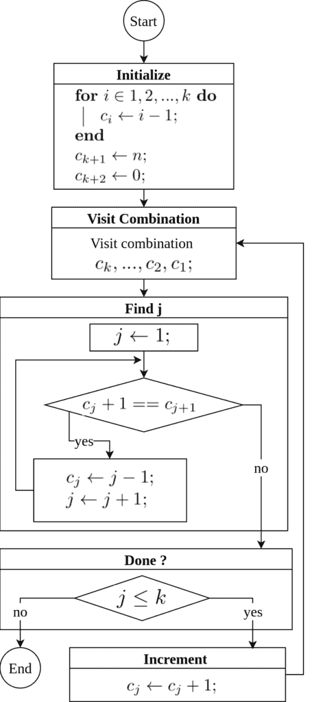
                visitCombination(c3, c2, c1)

In each iteration of the lexicographic generation algorithm, we find the smallest $j$ value, i.e., the rightmost element $c_j$ , that we can increment. Then we set the subsequent elements $c_{j-1},...,c_1$ to their smallest values.

For instance, when we have $n$ = 6 and $k$ = 3, the algorithm generates the lexicographically ordered sequence:

3. Filling a Rucksack Generation

We can formulate the $k$ -combinations as a Knapsack problem. Subsequently, an optimal solution involves visiting nodes in a binomial tree.

3.1. Binomial Trees

Binomial Trees is a tree family used in combination generation. They are denoted by $T_n$ for $n \geq 0$ , such that:

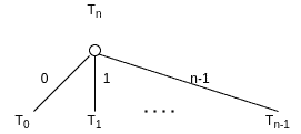
If $n$ =0, the tree $T_0$ consists of a single node
If $n>0$ , the binomial tree of order $n$ contains the root and $n$ binomial subtrees $T_{n-1},...,T_1,T_0$

For example, $T_4$ contains a root and subtrees $T_{3},T_2,T_1,T_0$ :

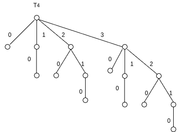
It’s easy to see that $T_n$ can be iteratively constructed from $T_{n-1}$ by inserting another copy of $T_{n-1}$ . So, $T_n$ contains $2^n$ nodes. Moreover, the number of nodes at each level $k$ equals to $\binom{n}{k}$ in $T_n$ for $k$ in {0,…, $n$ -1}. In this sense, the variations of Lexicographic generation algorithm traverses the nodes of $T_n$ on level $k$ .

3.2. Filling a Rucksack Algorithm

Let’s recall the 0-1 Knapsack Problem, where we either take or don’t take any element from a set of size ${n}$ to fill a rucksack. We can formulate our problem in a similar fashion, where we have a rucksack of size $\textbf{k}$ and we want to find all subset combinations of elements of set S. Let’s set $\delta_j = S_j - S_{j-1}$ for $1 \leq j < n$ . Subsets with number of elements $\leq k$ in the form $c_1,..,c_t$ are valid solutions to this problem.

In this case, every possible solution corresponds to a node of $T_n$ . We can use the following algorithm to visit each valid node in preorder:

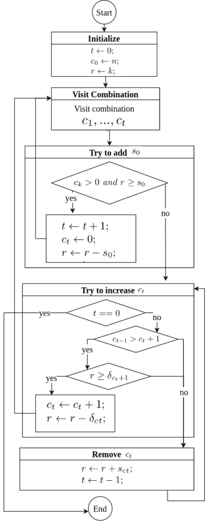
The algorithm only visits valid nodes of $T_n$ , skipping non-valid nodes. After the initialization phase, we visit the combination $c_1,...,c_t$ , using up $k - r$ space out of $k$ . Then we try to add elements to the combination at hand without exceeding the space restriction. If an element $c$ fits into a rucksack, we place it in after exhausting all possibilities using $c - 1$ in its place.

4. Revolving Door Generation

Another way to represent the $k$ -combinations problem is using Gray codes.

4.1. Gray Codes

Imagine a revolving door connecting two rooms. There are $k$ people in the left room and $n-k$ people on the right one. Hence, we have $n$ people in total. In this setting, we let a person go into the other room only by switching with somebody else, so that the number of people in the rooms never change:

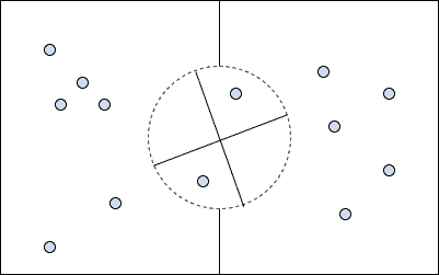
To represent the people in the rooms, we utilize $n$ bit binary strings. 0’s represent the people in the left room, and 1’s represent the people in the other room. Hence, 2 bits of a combination string bits are flipped when two people use the revolving door to switch places.

Let’s construct an algorithm to generate a sequence of combinations that don’t repeat. To generate such a sequence, we adopt Gray codes. We’ll enumerate orderings, where two successive representations always differ by one binary bit. Then, we’ll select only the binary representations containing $k$ zeroes and $n-k$ ones amongst them. Hence, the code sequence will satisfy the revolving door constraint.

By definition, we generate Gray binary codes of lenght $n$ recursively. Let $\Gamma_n$ represent a binary code of length $n$ . We canformulate it more formally as:

$\Gamma_n = 0\Gamma_{n-1}, 1\Gamma^R_{n-1}$

In other words, we generate Gray codes of length $n$ by inserting a leading 0 or 1 to Gray codes of length $n$ -1.

4.2. Revolving Door Algorithm

As our set has $\textbf{n}$ elements, we formulate a combination with a bit string of length $\textbf{n}$ . This string represents which elements to include in the combination with a 1, and not to include with a 0. To ensure we generate only the codes valid for the $k$ -combinations problem, we need to generate codes containing $n-k$ zeros and $k$ ones:

$\Gamma_{n-k,k} = 0\Gamma_{n-k-1,k}, 1\Gamma^R_{n-k,k-1}$

For instance, let’s consider the case $n$ =6 and $k$ =3. Let’s generate $\Gamma_{3,3}$ :

Converting the bit strings to combinations $c_3c_2c_1$ , we see a clear pattern:

In this sequence, $c_3$ occurs in increasing order. But for fixed values of $c_3$ , $c_2$ appears in increasing order. Moreover, for fixed $c_3c_2$ combinations, $c_1$ values are increasing again. So, we can say that the characters of combination alternatingly increase and decrease.

Putting it all together, we construct the revolving door algorithm to visit $\textbf{k}$ -combinations:

5. Near-Perfect Schemes and Perfect Schemes

We call a Gray path sequence homogeneous if only one $\textbf{c_j}$ is changed at each step. Since we have multiple indices changing simultaneously, the revolving door algorithm does not generate a homogeneous sequence. For instance, the transition from 210 to 320 or 432 to 420 doesn’t obey the homogeneity rule.

We can generate a homogenous Gray sequence for $n$ =6 and $k$ =3:

This bitstring corresponds to a homogenous sequence:

Even better, we can generate all ${k}$ -combinations by strongly homogenous transitions. In such a sequence, the $\textbf{c_j}$ index moves by at most 2 steps. These generation schemes are called near-perfect.

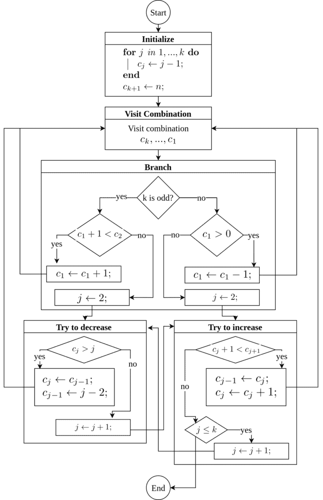
Chase formulated an easy to compute version of nearly-perfect sequences. Again, let’s say we have $n$ elements, and we want to find $k$ -combinations. Hence, we generate the binary sequence containing $k$ ones and $s = n-k$ zeros recursively:

As a result, we can use this algorithm to generate a sequence visiting all $\textbf{k}$ -combinations in near-perfect order. It’s called Chase’s sequence. There are exactly 2 $s$ such combinations.

Deducing from near-perfect combinations, we wonder if it’s possible to generate $\textbf{k}$ -combination sequences by only switching adjacent bits. This form is called a perfect scheme. Mathematicians proved that finding a perfect combination is possible only if $k \leq 1$ or $n-k \leq 1$ or $k \times (n-k)$ is odd. In short, finding a perfect scheme is possible in only 1 in 4 cases.

6. Comparison

In summary, the $k$ -combinations generation problem constructs elegant patterns. Heatmaps built with the binary outputs of the discussed strategies make these patterns easier to follow:

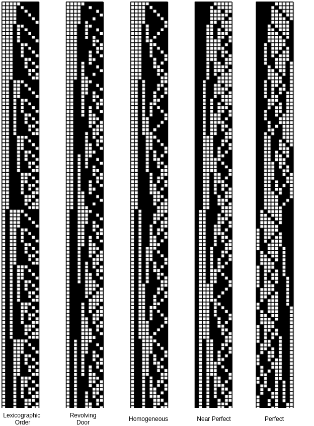
The image above was published in “The Art of Computer Programming”, volume 4A (2011).

7. Conclusion

In this article, we’ve learned about five different ways to enumerate ${k}$ -combinations of a set. Lexicographic order algorithm generates the subsets of size $k$ in alphabetical order, as the name suggests. The revolving door algorithm generates $k$ -combinations in alternating lexicographic order.

Homogeneous generation ensures that consecutive generations differ by only one element. Near-perfect schemes further ensure that the changed element moves at most two steps. Perfect schemes allow the changed element’s index to be incremented or decremented by only one.

Full Archive

About Baeldung

Core Concepts

Operating Systems

Artificial Intelligence

Graph Theory

Latex