0-1 Knapsack: A Problem With NP-Completeness and Solvable in Pseudo-Polynomial Time

1. Overview

The knapsack problem is an old and popular optimization problem. In this tutorial, we’ll look at different variants of the Knapsack problem and discuss the 0-1 variant in detail.

Furthermore, we’ll discuss why it is an NP-Complete problem and present a dynamic programming approach to solve it in pseudo-polynomial time.

2. General Definition

Given a knapsack with a weight limit of $W$ , a collection of $n$ items $x_1, x_2, x_3, ... , x_n$ with values $v_1, v_2, v_3, ..., v_n$ and weights $w_1, w_2, w_3, ..., w_n$ , the knapsack problem is defined as the optimization problem:

$\max \Sigma_{i=1}^{n} x_iv_i$

$\textrm{s.t.} \Sigma_{i=1}^{n} x_iw_i \leq W$

Now, the question is, what is the maximum value of the items that can be added to the knapsack such that the weight does not exceed the weight limit $\mathbf{W}$ ?

3. Variants of Knapsack Problem

There are three variants of the above knapsack problem depending on how $x_1, x_2, x_3, ..., x_n$ are defined. In this section, we’ll discuss these variants of this problem.

3.1. 0-1 Knapsack Problem

In this variant, the items are defined as: $x_i \in \{0,1\}, \ \forall\ i=1,2,..,n$

Here, there is only one of each item $i$ available. So if $x_i$ is $\mathsf{0}$ , that means the item is not added to the knapsack. If $x_i$ is $1$ , that means the item is added to the knapsack.

3.2. Bounded Knapsack Problem

In this case, the items are bounded by the condition: $0 \leq x_i \leq c, \ \forall\ i=1,2,..,n$

The variable $c$ denotes the number of available copies of each item.

3.3. Unbounded Knapsack Problem

Here, the items are in the form: $x_i \geq 0, \forall\ i=1,2,...,n$

In unbounded knapsack, there is no bound on the number of items. There are unlimited copies of each item available.

4. Why 0-1 Knapsack Problem Is NP-Complete?

The decision version of the 0-1 knapsack problem is an NP-Complete problem. Let’s see why.

Given weights and values of items, $W$ and $V$ , respectively, can a subset of items $X \subseteq \{1,2,..,n\}$ be picked that satisfy the following constraints:

$\Sigma_{i \in X} v_i \geq V$

$\Sigma_{i \in X} w_i \leq W$

A ‘Yes’ or ‘No’ solution to the above decision problem is NP-Complete. Solving the above inequalities is the same as solving the Subset-Sum Problem, which is proven to be NP-Complete. Therefore, the knapsack problem can be reduced to the Subset-Sum problem in polynomial time.

Further, the complexity of this problem depends on the size of the input values $v_i's$ , $w_i's$ . That is, if there is a way of rounding off the values making them more restricted, then we’d have a polynomial-time algorithm.

This is to say that the non-deterministic part of the algorithm lies in the size of the input. When the inputs are binary, it’s complexity becomes exponential, hence making it an NP-Complete problem.

5. Dynamic Programming Algorithm

In this section, we’ll discuss a dynamic programming approach for solving the 0-1 knapsack problem.

Let’s start by presenting its pseudocode:

Here, first, the algorithm creates a matrix of size $((n+1)\times (W+1))$ .

Every entry $M[i,w]$ denotes the maximum value the knapsack can take with a particular weight limit $w$ and $i$ items. We iterate over all possible weights (along the column) up to the weight limit $W$ and then pick a new item $i$ (next row) to see how the value of the knapsack increases.

To compute the maximum value at any given position in the matrix:

If $w_i > w$ : $\ M[i,w] = M[i-1,w]$
If $w_i \leq w$ : $M[i,w] = max(M[i-1,w-w_i]\ +\ v_i,\ M[i-1,w])$

The function $M[i-1, w]$ denotes the value at the position right above the current position $(i-1, w)$ , to check without adding the item $i$ , and $M[i-1,w-w_i]+v_i$ presents the value of the knapsack if the current item is added.

A general idea is to pick the current item, which is the $i^{th}$ item (for a given weight limit $w$ if the first term in the $max()$ function above is more than the second). The second term represents the total value at weight capacity $w$ if we do not pick the $i^{th}$ item.

6. An Example

Now, as we are done discussing the dynamic approach for the 0-1 knapsack problem, let’s run the algorithm on an example:

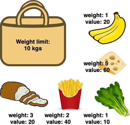
We can only carry $10kgs$ in our grocery bag. We’re interested in finding what would be the maximum value (say calories here) of all the items in the bag combined.

For this example, we’ve already defined the weights and values:

$W = \{1,2,1,3,5\}$

$V = \{10,40,20,20,60\}$

Now, according to the algorithm, the first step is to initialize the matrix, $M$ , with the first row and the first column entries to zeros.

After the initialization of the matrix $M$ , it’s time to start the iteration step.

Let’s start the first loop. For the values: $i = 1,\ w=1,\ w_i=1,\ v_i=10,\ w_i \leq w$ :

$M[1,1] = max(M[0,0] + 10,\ M[0,1])$

$M[1,1] = 10$

It can be verified that $M[1,w] = 10$ for $2 \leq w \leq 10$ because $w_1 \leq w$ in that interval:

$M[1,w] = max(M[0,w-w_1] + 10, M[0,w])$

$M[0,w] = 0,\ M[0,w-w_1]=0\ \forall\ 2 \leq w \leq 10$

Let’s discuss the result in the table. Our first column is $\mathsf{0}$ . It denotes that if the total weight is $\mathsf{0}$ , no matter what item we choose, the maximum knapsack value is always $\mathsf{0}$ .

Next, we choose the weight equals $1$ . With the value of $10$ , the maximum we can get is $10$ . So we filled all the rows with a maximum knapsack value of $10$ .

Now, let’s start the second loop.

For the values $i = 2,\ w=1,\ w_i=2,\ v_i=40,\ w_i > w$ :

$M[2,1] = M[1,1]$

For the other values, we’ll increase the value of $w$ and keep everything else unchanged. We’ll start the loop with the values $i = 2,\ w=2,\ w_i=2,\ v_i=40,\ w_i \leq w$ :

$M[2,2] = max(M[1,0] + 40,\ M[1,2]) = max(40,10) = 40$

Inside the $max$ function were two choices – to either pick item # $2$ (in such case, the value of item # $2$ gets added) or to leave it.

Again, for $i = 2,\ w=3,\ w_i=2,\ v_i=40,\ w_i \leq w$ :

$M[2,3] = max(M[1,1] + 40,\ M[1,3]) = max(10+40,10) = 50$

$M[2,w] = 50,\ \forall\ 4 \leq w \leq 10$ because $w_2 \leq w$ in that interval:

$M[2,w] = max(M[1,w-w_2] + 40, M[1,w])$

$M[1,w] = 10, M[1,w-w_2] = 10\ \forall\ 4 \leq w \leq 10$

In this table, when the capacity is $1$ and the weight of the item is $2$ , we can’t choose the item. Therefore, the maximum knapsack value won’t update when capacity is equal to $1$ . For the rest of the capacity values, the maximum knapsack capacity values are updated by the formula.

Let’s continue the iteration and increase the value of $i$ . For the values $i = 3,\ w=1,\ w_i=1,\ v_i=20,\ w_i \leq w$ :

$M[3,1] = max(M[2,0] + 20, M[2,1]) = max(20,10) = 20$

Now, we need to increase the value of $w$ and run the loop $i = 3,\ w=(2, 3, 4)\ w_i=1,\ v_i=20,\ w_i \leq w$ :

$M[3,2] = max(M[2,1] + 20, M[2,2]) = max(10+20,40) = 40$

$M[3,3] = max(M[2,2] + 20, M[2,3]) = max(40+20,50) = 60$

$M[3,4] = max(M[2,3] + 20, M[2,4]) = max(50+20,50) = 70$

Here, the weight $= 1$ . Therefore, we choose this item and update all the values in the row.

Let’s continue the iteration. Now, for the values $i = 4,\ w=1,\ w_i=3,\ v_i=20,\ w_i > w$ :

$M[4,1] = M[3,1] = 20$

Again, for the values $i = 4,\ w=(2, 3, 4, 5, 6, 7, 8, 9, 10)\ w_i=3,\ v_i=20,\ w_i \leq w$ :

$M[4,2] = M[3,2] = 40$

$M[4,3] = max(M[3,0] + 20, M[3,3]) = max(20,60) = 60$

$M[4,4] = max(M[3,1] + 20, M[3,4]) = max(20+20,70) = 70$

$M[4,5] = max(M[3,2] + 20, M[3,5]) = max(40+20,70) = 70$

$M[4,6] = max(M[3,3] + 20, M[3,6]) = max(60+20,70) = 80$

$M[4,7] = max(M[3,4] + 20, M[3,7]) = max(70+20,70) = 90$

$M[4,8] = max(M[3,5] + 20, M[3,8]) = max(70+20,70) = 90$

$M[4,9] = max(M[3,6] + 20, M[3,9]) = max(70+20,70) = 90$

$M[4,10] = max(M[3,7] + 20, M[3,10]) = max(70+20,70) = 90$

The current weight here is $3$ . So, for the capacity values $1$ and $2$ , we can’t select this item. Hence, for capacity $1$ and $2$ , the maximum knapsack capacity values are unchanged. For the other capacity values, we do select the item and change the maximum capacity values.

It’s time to increase the value of $i$ and run the iteration. Therefore, the values in the loop $i = 5,\ w=1,\ w_i=5,\ v_i=60,\ w_i > w$ :

$M[5,1] = M[4,1] = 20$

We need to increase the value of $w$ , and everything else is unchanged. Hence, for $i = 5,\ w=(2, 3, 4, 5, 6, 7, 8, 9, 10)\ w_i=5,\ v_i=60,\ w_i > w$ :

$M[5,2] = M[4,2] = 40$

$M[5,3] = M[4,3] = 60$

$M[5,4] = M[4,4] = 70$

$M[5,5] = max(M[4,0] + 60, M[4,5]) = max(60,70) = 60$

$M[5,6] = max(M[4,1] + 60, M[4,6]) = max(20+60,80) = 80$

$M[5,7] = max(M[4,2] + 60, M[4,7]) = max(40+60,90) = 100$

$M[5,8] = max(M[4,3] + 60, M[4,8]) = max(60+60,90) = 120$

$M[5,9] = max(M[4,4] + 60, M[4,9]) = max(70+60,90) = 130$

$M[5,10] = max(M[4,5] + 60, M[4,10]) = max(70+60,90) = 130$

Lastly, when the weight of the item is $5$ , we can update the values for which capacity value $\geq$ $5$ .

Finally, we’re done with the iterations. We end up with the result that when the weight limit is $\textbf{10}$ kgs, the maximum knapsack value is $\textbf{130}$ .

7. Time Complexity Analysis

Let’s analyze the time complexity of the dynamic programming algorithm in this section.

The first two initializations of function $M[ ]$ can be done in $\mathcal{O}(1)$ time. The for loop that iterates from $1$ to $n$ takes $\mathcal{O}(n)$ time. Under this, there is another for loop which goes from $1$ to $W$ . It takes $\mathcal{O}(W)$ time. Finally, the $max()$ can be computed in $\mathcal{O}(1)$ time.

Therefore, a 0-1 knapsack problem can be solved in $\mathcal{O}\mathbf{(nW)}$ using dynamic programming. It should be noted that the time complexity depends on the weight limit of $W$ .

Although it seems like it’s a polynomial-time algorithm in the number of items $n$ , as W increases from say 100 to 1,000 ( $\sim2^7$ to $\sim2^{10}$ ), processing $W$ goes from $7$ bits to $10$ bits. The time complexity increases exponentially with the number of bits.

For example, if the weight $W$ is not large, then the complexity can be perceived as polynomial time in the number of input items, hence the term “pseudo-polynomial”.

8. Conclusion

In this article, we’ve discussed the 0-1 knapsack problem in depth. We’ve explained why the 0-1 Knapsack Problem is NP-complete.

For solving this problem, we presented a dynamic programming-based algorithm. We ran the algorithm on an example problem to ensure the algorithm is giving correct results. Finally, we analyzed the time taken by the dynamic algorithm.

Full Archive

About Baeldung

Core Concepts

Operating Systems

Artificial Intelligence

Graph Theory

Latex