

Learn through the super-clean Baeldung Pro experience:
>> Membership and Baeldung Pro.
No ads, dark-mode and 6 months free of IntelliJ Idea Ultimate to start with.
Learn through the super-clean Baeldung Pro experience:
>> Membership and Baeldung Pro.
No ads, dark-mode and 6 months free of IntelliJ Idea Ultimate to start with.
In this article, we’ll explore Differential Evolution (DE), renowned for addressing complex optimization problems across various domains. Additionally, we’ll discuss the algorithm’s functionality, effectiveness, and applications, emphasizing its robustness and versatility in tackling intricate challenges.
Differential Evolution is a smart search algorithm that improves potential solutions repeatedly to optimize problems, similar to how evolution operates.
Rainer Storn and Kenneth Price developed it back in the mid-1990s. Since then, the Differential Evolution has become popular for tackling tough optimization problems in different areas. People like it because it’s strong, flexible, and works well in many situations.
Differential Evolution (DE) functions as a nature-inspired search strategy within the broader category of evolutionary computation, encompassing a variety of optimization algorithms that draw inspiration from natural selection and genetics. To understand DE better, let’s look at the related concept of genetic algorithms (GA), a prominent member of the evolutionary computation family:
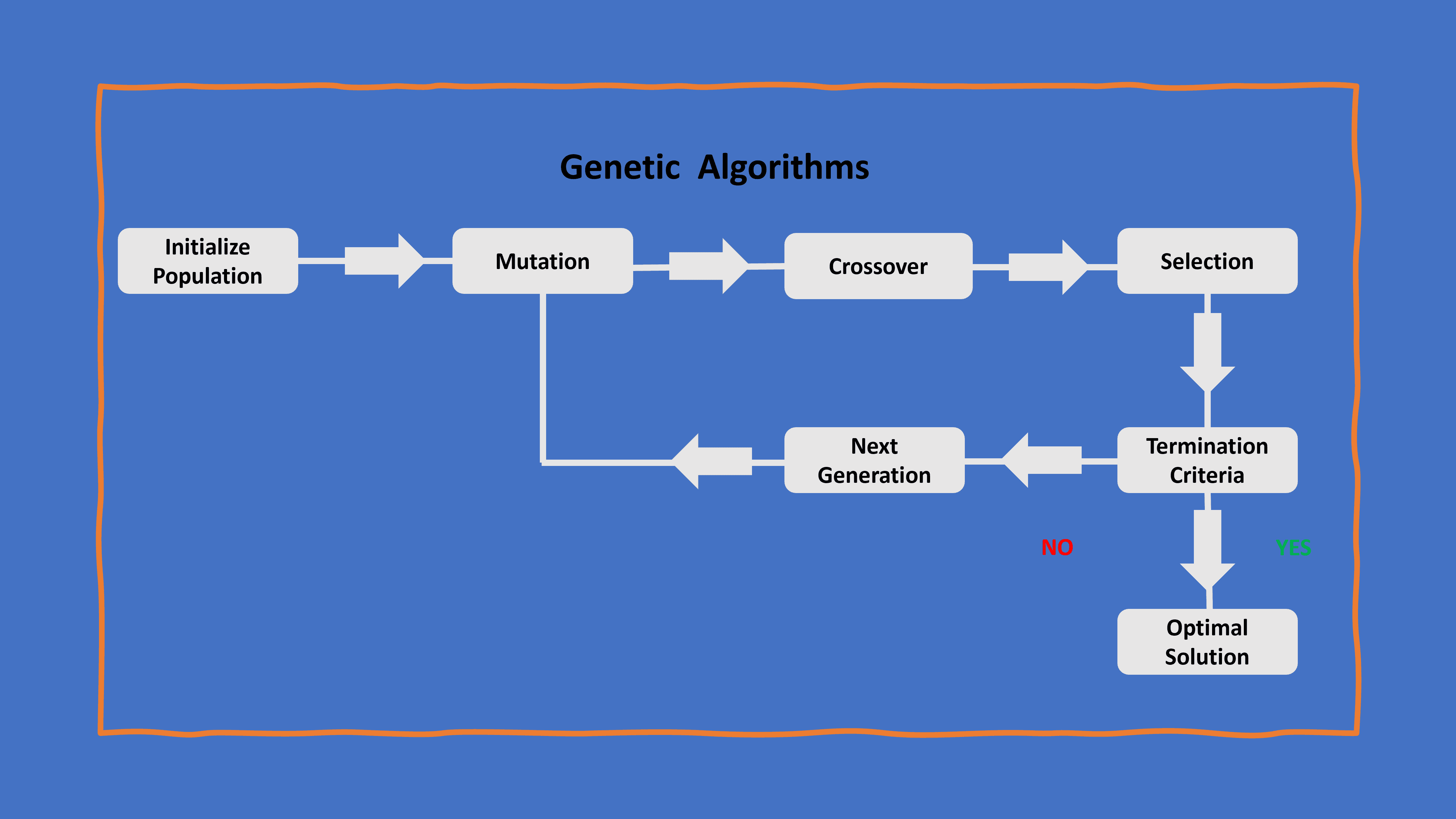
In genetic algorithms, the population treats individuals as candidate solutions, applies genetic operations (crossover and mutation) to them, and assesses their fitness. The principles guiding genetic algorithms lay the groundwork for comprehending the population-based optimization approach employed by DE.
Differential Evolution operates on a population of candidate solutions, setting it apart from traditional optimization methods that focus on a single solution. This population-based approach fosters diversity and facilitates thoroughly exploring the solution space. Leveraging three key operations: mutation, crossover, and selection, DE iteratively evolves the population towards optimal solutions.
While population-based operation is a fundamental characteristic of Differential Evolution, it’s noteworthy that many other evolutionary algorithms share this trait.
In genetic algorithms, we treat possible solutions as individuals in a group. These individuals undergo genetic operations like crossover and mutation, and then we evaluate their performance. The ideas behind genetic algorithms help us grasp the population-based optimization method used by DE.
Genetic Algorithms and Differential Evolution are two distinct evolutionary optimization algorithms with differing approaches to solving optimization problems.
In GAs, individuals in the population are typically represented as binary or integer strings, and the algorithm employs crossover and mutation operators to create offspring for subsequent generations.
DE, on the other hand, operates on vectors of real numbers, using a unique differential mutation strategy that combines vectors to generate trial vectors. DE’s population update is more gradual, replacing individuals based on their performance compared to trial vectors. While GAs often use traditional selection mechanisms, DE introduces a different selection strategy. DE is known for its faster convergence, particularly in high-dimensional optimization problems, making it effective in scenarios where GAs may face challenges.
Differential Evolution comprises three key components that collectively contribute to its effectiveness in solving complex optimization problems.
The first step in DE is getting things going. We start by creating a bunch of possible solutions randomly. Each solution is like a guess at the answer to the problem we’re trying to solve.
Here’s the pseudocode:
algorithm InitializePopulation(populationSize, solutionDimension):
    // INPUT
    //     populationSize = the size of the initial population
    //     solutionDimension = the dimension of the solution space
    // OUTPUT
    //     the initial population

    population <- an empty set

    // Create individuals for the population
    for i in [1, ..., population_size + 1]:
        individual <- generate a random solution
        population[i] <- individual

    return population
Here’s where DE stands out. This operation involves a strategic combination of information from three randomly selected individuals within the population. This unique mutation strategy is a defining characteristic of DE, playing a crucial role in introducing diversity into the population.
Here’s the pseudocode:
algorithm MutationOperation(population, mutationFactor):
    // INPUT
    //     population = the current population of individuals
    //     mutationFactor = a factor determining the extent of mutation
    // OUTPUT
    //     mutatedPopulation = the population after mutation

    mutatedPopulation <- an empty set

    // Iterate through each individual in the population
    for target in population:
        a, b, c <- randomly select three distinct individuals for mutation

        // Mutate the target individual based on the differences
        mutatedIndividual <- target + mutationFactor * (a - b + c)

        // Add the mutated individual to the population
        mutatedPopulation.append(mutatedIndividual)

    return mutatedPopulation
For instance, let’s consider a scenario in which DE optimizes the parameters of a machine-learning model. Each individual in the population represents a set of parameter values, and the mutation operation involves perturbing these parameters based on the differences between three randomly chosen individuals. This process introduces variations that aid in exploring the solution space effectively.
The crossover part is crucial too. It takes the best solution from the group (called the target) and combines it with the changes we made earlier (from the mutation). This creates a new configuration, like mixing and matching the best parts. In a real-world example, if we’re optimizing a production process, the target might be a specific set of operating conditions, and the mutation introduces some changes. The crossover then blends these, and we check how well it works based on our goals, like making things more efficient or reducing production time.
Here’s the pseudocode:
algorithm CrossoverOperation(population, crossoverRate):
    // INPUT
    //     population = the current population of individuals
    //     crossoverRate = the probability of crossover
    // OUTPUT
    //     crossedPopulation = the population after crossover

    crossedPopulation <- an empty set

    // Iterate through each individual in the population
    for i in [1, ..., length(population)]:
        // Randomly select a target individual
        target <- population[i]

        // Apply crossover with the target and a randomly chosen mutant
        if uniform random number < crossoverRate:
            mutantIndex <- randomly select an index that is not i
            mutant <- population[mutantIndex]
            crossedIndividual <- Crossover(target, mutant)
        else:
            crossedIndividual <- target

        // Add the crossed individual to the population
        crossedPopulation.append(crossedIndividual)

    return crossedPopulation

algorithm Crossover(target, mutant):
    // INPUT
    //     target = the target individual for crossover
    //     mutant = the mutant individual for crossover
    // OUTPUT
    //     crossed individual resulting from the crossover

    // Placeholder logic
    crossed <- CrossoverLogic(target, mutant)

    return crossed
So, in simple terms, DE starts with random guesses, shakes things up in a smart way, and then combines the best elements to find the optimal solution for a given problem.
DE employs a selection mechanism to determine whether the trial vector should replace the target vector in the population. The decision depends on evaluating the fitness of the trial vector using the objective function. The selection mechanism is crucial for driving the evolutionary process towards improved solutions.
Here’s the pseudocode:
algorithm SelectionMechanism(population, mutatedPopulation, objectiveFunction):
    // INPUT
    //     population = the current population of individuals
    //     mutatedPopulation = the population after mutation
    //     objectiveFunction = the function used to evaluate the fitness of individuals

    // OUTPUT
    //     selectedPopulation = the population after selection

    selectedPopulation <- an empty set

    // Iterate through each individual in the population
    for i in [1, ..., length(population)]:
        // Evaluate the fitness of the target and trial vectors using the objective function
        targetFitness <- objectiveFunction(population[i])
        trialFitness <- objectiveFunction(mutatedPopulation[i])

        // Replace the target vector with the trial vector if it is better
        if trialFitness < targetFitness:
            selectedIndividual <- mutatedPopulation[i]
        else:
            selectedIndividual <- population[i]

        // Add the selected individual to the population
        selectedPopulation.append(selectedIndividual)

    return selectedPopulation
For instance, In the optimization of a logistics network, each individual in the population represents a distribution plan. The selection mechanism assesses the fitness of the trial distribution plan based on factors like cost and delivery time. If the trial plan outperforms the existing one, it replaces the target plan in the population, influencing subsequent generations to converge toward more optimal logistics solutions.
Understanding the nuances of these key components provides insights into how DE operates and adapts populations over successive generations, ultimately converging towards solutions that meet predefined optimization objectives.
The algorithmic workflow of the Differential Evolution encompasses key stages that govern its operation, from initializing the population to determining the termination conditions.
Here’s a step-by-step breakdown of the Differential Evolution algorithm:
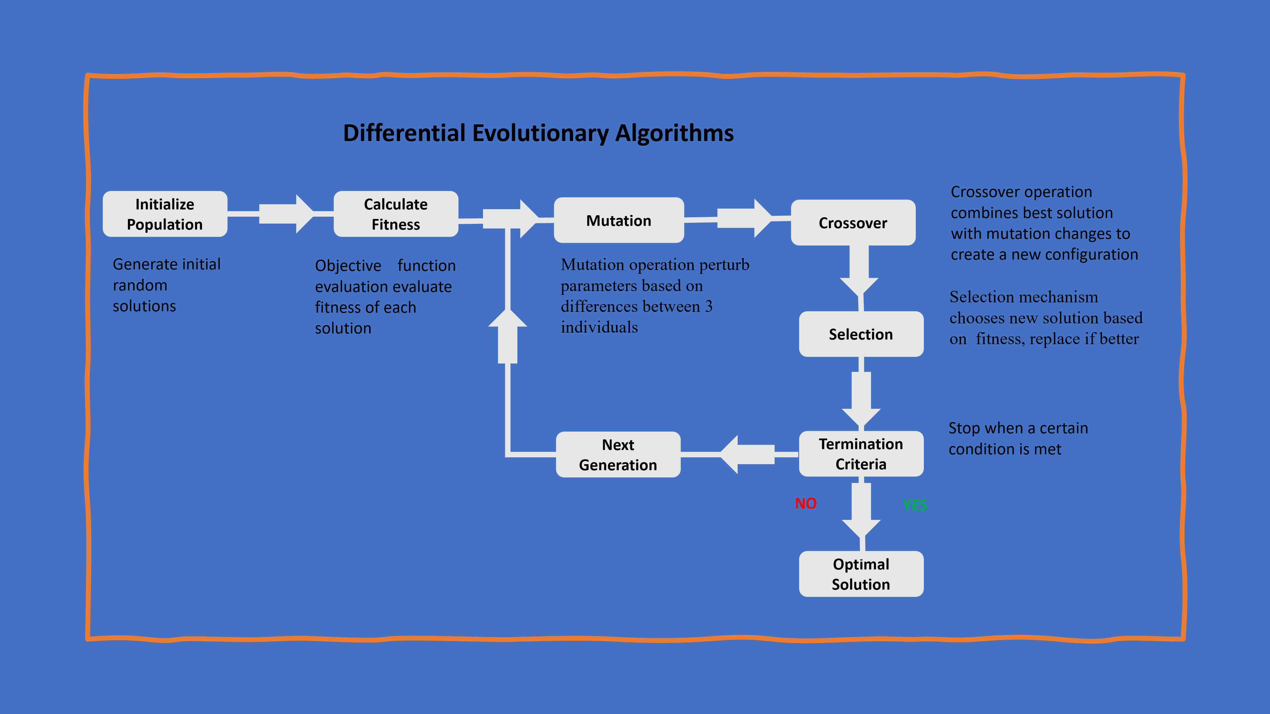
The DE algorithm kicks off its execution by generating an initial population consisting of candidate solutions. These solutions represent potential configurations or individuals within the solution space that will undergo evolutionary processes.
In a real-world application, if one uses DE to optimize the layout of a manufacturing facility, the initialization step involves creating an initial set of diverse layouts.
DE follows an iterative process wherein the algorithm evolves the population over successive generations. This involves the application of mutation, crossover, and selection operations. The iterative nature allows DE to progressively refine candidate solutions toward optimal configurations.
For example, continuing with the manufacturing facility layout optimization, during each iteration, DE could adjust the positions of machines (mutation), combine features of different layouts (crossover), and select layouts based on their performance (selection).
The termination criteria dictate when the DE algorithm concludes its execution. The algorithm can sufficiently explore the solution space after a specified number of generations or when it meets a convergence criterion.
For instance, if someone uses DE to optimize the scheduling of tasks in a project, the algorithm might conclude when it reaches a set number of scheduling generations or when the project schedule converges to an optimal solution, satisfying predefined criteria.
Understanding the algorithmic workflow, from initialization through the iterative process to termination, is pivotal for grasping how Differential Evolution systematically refines its solutions to approach optimal configurations.
Here’s the pseudocode:
algorithm DifferentialEvolutionAlgorithm(initialState, maxIteration, convergenceCriteria, mutationFactor, crossoverRate):
    // INPUT
    //     initialState = the initial state or population
    //     maxIteration = the maximum number of iterations
    //     convergenceCriteria = the criteria for convergence
    //     mutationFactor = a factor determining the extent of mutation
    //     crossoverRate = the probability of crossover

    // OUTPUT
    //     bestIndividual = the best individual found by the algorithm

    currentGeneration <- initialState
    i <- 0

    // Iterate until convergence or reaching the maximum iteration
    while not ConvergenceMet(currentGeneration, convergenceCriteria) and i <= maxIteration:
        i += 1

        // Perform mutation and create donor vectors
        donorVectors <- PerformMutation(currentGeneration, mutationFactor)

        // Perform crossover and create trial vectors
        trialVectors <- PerformCrossover(currentGeneration, donorVectors, crossoverRate)

        // Select the next generation
        currentGeneration <- SelectNextGeneration(currentGeneration, trialVectors)

    // Find the best individual in the final generation
    bestIndividual <- FindBestIndividual(currentGeneration)

    return bestIndividual
The Differential Evolution Algorithm (DE) offers several advantages that contribute to its effectiveness in solving complex optimization problems. Specifically, we compare DE to a broader class of optimization techniques rather than specifically to other evolutionary algorithms.
| Advantage | Description |
|---|---|
| Global Search Capability | DE excels in exploring diverse solution spaces, making it suitable for complex, non-linear problems. |
| Few Tunable Parameters | DE typically requires fewer parameter adjustments, enhancing its user-friendliness. |
| Robustness | DE is less sensitive to parameter choices and performs well in noisy and dynamic environments. |
| Versatility | Applicable across various domains, including machine learning, engineering, and finance. |
| Population-Based Approach | DE’s population-based optimization allows for the simultaneous exploration of multiple solutions. |
Differential Evolution (DE) finds diverse applications across various domains due to its robustness and effectiveness in solving optimization problems. Let’s explore practical examples:
The Differential Evolution Algorithm finds extensive application in engineering optimization tasks. For instance, in the design of aerodynamic shapes for aircraft, DE can efficiently optimize parameters such as wing profiles to enhance performance metrics like lift and drag.
This active approach ensures that the resulting designs meet or exceed specified criteria, contributing to the efficiency of engineering processes.
In the realm of machine learning, DE plays a crucial role in training neural networks. By optimizing the weights and biases of the network, DE ensures that the model accurately captures patterns in data.
For example, DE actively refines the neural network’s parameters in image recognition to improve its ability to identify and classify objects, contributing to the model’s overall performance.
In game development, developers use DE to optimize strategies in competitive games. For instance, in designing non-player character (NPC) behaviors, DE actively refines decision-making algorithms to create more challenging and dynamic opponents.
This application ensures an engaging and active gaming experience for players.
Financial sectors widely use DE to optimize investment portfolios. By adjusting the allocation of assets based on historical data and risk preferences, DE helps investors create portfolios that maximize returns while managing risk. For instance, in portfolio optimization, DE actively selects the optimal mix of stocks, bonds, and other assets to achieve desired financial goals.
In general, these examples illustrate the active role of the Differential Evolution Algorithm across various domains, showcasing its versatility and effectiveness in solving complex optimization challenges.
In this article, we explored the versatile applications and key advantages of Differential Evolution. DE’s active role in solving complex optimization problems is evident across diverse domains, showcasing its efficiency in engineering, finance, machine learning, and game development. Its global search capability, minimal parameter tuning requirements, and population-based approach contribute to its effectiveness in real-world scenarios.
In conclusion, Differential Evolution stands as a robust and adaptable tool, offering tangible benefits in refining solutions for intricate challenges. DEA’s active approach and versatility position it as a valuable asset, making a significant impact in optimizing processes across engineering, finance, and beyond.