

Learn through the super-clean Baeldung Pro experience:
>> Membership and Baeldung Pro.
No ads, dark-mode and 6 months free of IntelliJ Idea Ultimate to start with.
Learn through the super-clean Baeldung Pro experience:
>> Membership and Baeldung Pro.
No ads, dark-mode and 6 months free of IntelliJ Idea Ultimate to start with.
Evolutionary algorithms have been a subject of study in machine learning for decades. They comprise a large family of techniques such as genetic algorithms, genetic programming, evolutionary programming, and so on. They can be applied to a variety of problems, from variable optimization to new designs in building a tool like an antenna. In this article, we highlight some of the impressive techniques and algorithms that have stood out.
A typical evolutionary algorithm has the following workflow:
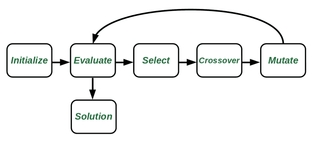
Knowing the jargon used in the context of evolutionary algorithms can help us grasp the ideas more easily. A population is a set of candidates for the solution, and its representation is called genotype. A generation is a step in the process where evolutionary operations take place on the population.
Operations for creating new candidate solutions include selection, crossover, and mutation. By selecting the best-performing individuals to move to the next generation, crossover exploits different combinations of the individuals, and mutation finds and explores new directions. Finally, there’s a fitness function (objective) that measures how close the results are to a specified goal.
In radio communications, sometimes there’s a need for designing an antenna with unusual radiation patterns for a particular mission. However, its design is not possible manually since there is an enormous number of patterns to try out. In such cases, an evolutionary algorithm comes in handy.
The 2006 NASA ST5 spacecraft antenna makes use of one of these algorithms:
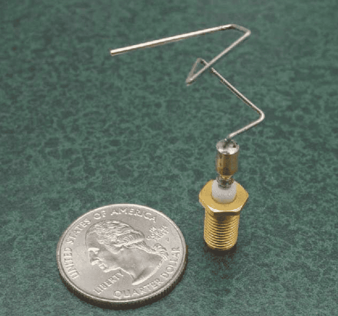
In order to build this antenna, the process starts with an initial feed wire of length 0.4 cm along the Z-axis. Then, there are four operations that control its growth. These are  ,
,  ,
,  , and
, and  . The
. The  operation adds wire with the given length and radius to the current state location. The other three control the direction in which the antenna grows.
In every step (generation), the fitness function, which is the product of 3 factors, measures the performance of the model:
![\[ F = vswr \times gain_{error} \times gain_{smoothness} \]](/wp-content/ql-cache/quicklatex.com-8a2e067e737ea45209a1e7f0da85712a_l3.svg "Rendered by QuickLaTeX.com")
where  is the measure of impedance matching between the antenna and the transmission line it is connected to. The
  factor is a modified version of the least squared error, and the
  is to ensure that the antennas produce smooth gain patterns. It is the weighted sum of the standard deviation of gain values for each elevation angle.
Minimizing the fitness function leads to the creation of the unusually shaped antenna, which outperforms the handmade ones.
One of the recently emerging areas in artificial intelligence is the Neural Architecture Search (NAS). It studies the automation of neural network design. For a (deep) neural network, there is a multitude of hyperparameters for optimizing its performance. Examples are the number of layers, learning rate, different architecture modules, and so on. This means that there is a large search space that we need to explore, an area that evolutionary algorithms specialize in.
Recently, a study from the Google Brain team showed that using an evolutionary algorithm, image classifiers can achieve state-of-the-art results. They start with a population of random architectures. Then, within a specific number of cycles, each time, they draw a random sample of the population uniformly and choose the one with the highest validation fitness. After that, they apply a simple transformation to the chosen one using mutations.
Finally, they train and evaluate the new model and add it to the population. In contrast to traditional methods, each time a new model is added to the population, they discard the oldest one instead of the worst one. By doing this, they favor exploring the search space more and avoid the models that are good in the early stages.
The mutations adopted by them are threefold:
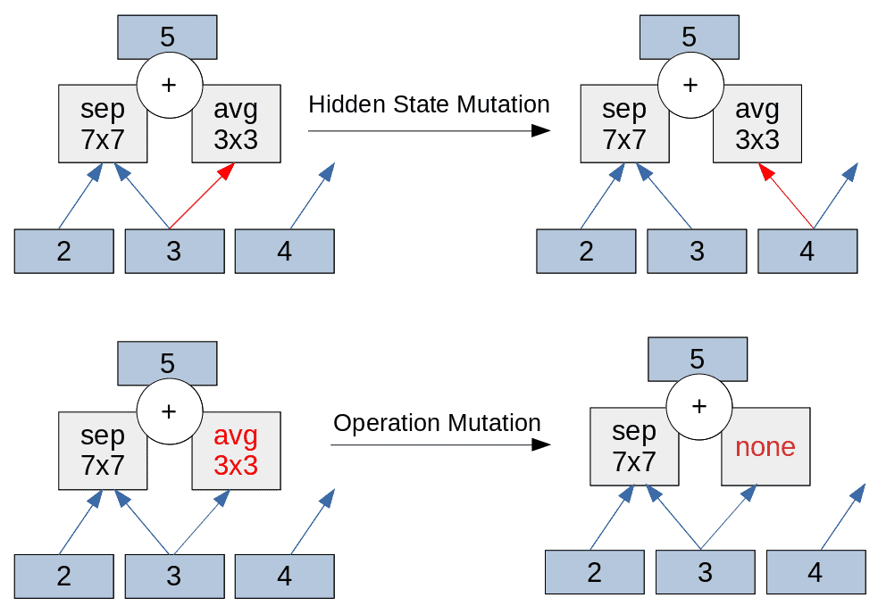
In the figures, the numbered squares represent a hidden state. The hidden state mutations consist of choosing, first, one type of cell ( or
or  ) and then one of the five pairwise combinations. Normal and reduction cells have the same architecture with a different stride (2 for reduction) in order to reduce the image size while the normal cell keeps the image size. After selecting the pairwise combination, they choose one of its two elements and replace its hidden state with another from the same cell.
The mutation of the operation is similar to that of the hidden state in terms of its necessary elements with the difference that, this time, the operation is replaced instead of the hidden state. The possible operations are separable convolutions with three different kernel sizes, average pooling, max pooling, and dilated convolutions.
A third mutation is also possible, which is the identity (none) and the fitness objective of the model is the loss function of the classifier to minimize.
Reinforcement learning in AI is developing fast because of its effectiveness in areas where there’s an interaction between the algorithm and the environment. However, they can be complex and slow due to the back-propagation process and difficulty in parallelizing the computations.
Evolution strategies do away with these problems by having only a forward pass and their ability to be parallelized. A study by a research team from the Open AI company showed that an algorithm based on evolution strategies could achieve a close performance to reinforcement learning algorithms on optimization tasks.
Their strategy is really simple. Let’s assume that the model we want to optimize has some parameters  . Then the reward function will be
  for which we want to find the optimal value. We start by assigning random values to the parameter vector . Then, we generate a number (e.g., 100) of slightly different vectors from the parent vector by adding Gaussian noise to it.
After that, we evaluate each of the resulting vectors and create a new one by combining all the previous vectors with their obtained rewards as their (proportional) weights in the combination. As a result, we favor the ones that produce better rewards. Finally, the fitness function is the expected reward of the model.
In this tutorial, we reviewed some of the evolutionary algorithms that have performed well compared to other techniques in artificial intelligence.